Effect of variable surrounding on species creation

Aleksandra Nowicka; Artur Duda; Mirosław R. Dudek

doi:10.1016/j.crvi.2003.11.011

Biological modelling / Biomodélisation

Effect of variable surrounding on species creation
[Effet d'un milieu variable sur l'apparition des espèces]

Présenté par : Pierre Auger

Aleksandra Nowicka ¹ ; Artur Duda ² ; Mirosław R. Dudek ³

¹ Institute of Microbiology, University of Wrocław, ul. Przybyszewskiego 63/77, 54-148 Wrocław, Poland
² Institute of Theoretical Physics, University of Wrocław, pl. Maxa Borna 9, 50-204 Wrocław, Poland
³ Institute of Physics, Zielona Góra University, 65-069 Zielona Góra, Poland

Comptes Rendus. Biologies, Volume 327 (2004) no. 3, pp. 283-292.

Résumés

Anglais
Français

We constructed a model of speciation from evolution in an ecosystem consisting of a limited amount of energy recources. The species possesses genetic information, which is inherited according to the rules of the Penna model of genetic evolution. The increase in the number of the individuals of each species depends on the quality of their genotypes and the available energy resources. The decrease in number of the individuals results from genetic death or maximum-age reaching by the individual. The amount of energy resources is represented by a solution of the differential logistic equation, where the growth rate of the amount of the energy resources has been modified to include the number of individuals from all species in the ecosystem under consideration.

The fluctuating surrounding is modelled with the help of the function $V (x, t) = \frac{1}{4} x^{4} + \frac{1}{2} b (t) x^{2}$ , where x represents phenotype and the coefficient b(t) shows the cos(ωt) time dependence. The closer the value x of an individual to the minimum of V(x,t), the better adapted its genotype to the surrounding. We observed that the life span of the organisms strongly depends on the value of the frequency ω. It becomes shorter the more frequent the changes of the surrounding. However, there is a tendency for the species that have a higher value of the reproduction age a_R to win the competition with the other species.

Another observation is that small evolutionary changes of the inherited genetic information lead to spontaneous bursts of the evolutionary activity when many new species may appear in a short period.

. Un modèle de spéciation issu de l'évolution dans un écosystème aux ressources énergétiques limitées a été créé. Les espèces possédent des informations génétiques qui sont héritées selon les règles du modèle de Penna d'evolution génétique. L'augmentation du nombre d'individus de chaque espèce dépend de la qualité de leur génotype et de l'accessibilité des ressources énergétiques. La diminution du nombre d'individus résulte de la mort génétique ou de l'arrivée de l'un d'entre eux à l'âge maximum. La quantité des ressources énergétiques est donnée par la résolution de l'équation différentielle logique, où le taux de renouvellement de la quantité de ressources énergétiques a été modifié pour tenir compte de la quantité d'individus de toutes les espèces de l'écosystème analysé.

Les fluctuations du milieu sont modélisées par la fonction $V (x, t) = \frac{1}{4} x^{4} + \frac{1}{2} b (t) x^{2}$ , où x représente un phénotype et le coefficient b(t) désigne cos(ωt), la dépendance temporelle. Plus la valeur x d'un individu est proche du minimum V(x,t), mieux son génotype est adapté au milieu. Il a été constaté que la durée de vie des organismes dépend fortement de la valeur de la fréquence ω. Plus les changements du milieu sont fréquents, plus celle-ci devient faible. Cependant, les espèces dont la valeur a_R de l'âge de reproduction est élevée ont tendance à remporter la compétition avec les autres espèces.

L'autre observation est que les petits changements évolutifs des informations génétiques héritées conduisent à des explosions spontanées de l'activité évolutive, et de nombreuses nouvelles espèces peuvent alors apparaître, dans un laps de temps court.

Métadonnées

Reçu le : 2003-04-15
Accepté le : 2003-11-26
Publié le : 2004-03-01

PMID

DOI : 10.1016/j.crvi.2003.11.011

Keywords: speciation, ecosystem, genetic evolution, Penna model, Lotka–Volterra model
Mot clés : spéciation, écosystème, évolution génétique, modèle de Penna, modèle de Lotka–Volterra

Affiliations des auteurs :

Aleksandra Nowicka ¹ ; Artur Duda ² ; Mirosław R. Dudek ³

¹ Institute of Microbiology, University of Wrocław, ul. Przybyszewskiego 63/77, 54-148 Wrocław, Poland
² Institute of Theoretical Physics, University of Wrocław, pl. Maxa Borna 9, 50-204 Wrocław, Poland
³ Institute of Physics, Zielona Góra University, 65-069 Zielona Góra, Poland

@article{CRBIOL_2004__327_3_283_0,
     author = {Aleksandra Nowicka and Artur Duda and Miros{\l}aw R. Dudek},
     title = {Effect of variable surrounding on species creation},
     journal = {Comptes Rendus. Biologies},
     pages = {283--292},
     publisher = {Elsevier},
     volume = {327},
     number = {3},
     year = {2004},
     doi = {10.1016/j.crvi.2003.11.011},
     language = {en},
}

TY  - JOUR
AU  - Aleksandra Nowicka
AU  - Artur Duda
AU  - Mirosław R. Dudek
TI  - Effect of variable surrounding on species creation
JO  - Comptes Rendus. Biologies
PY  - 2004
SP  - 283
EP  - 292
VL  - 327
IS  - 3
PB  - Elsevier
DO  - 10.1016/j.crvi.2003.11.011
LA  - en
ID  - CRBIOL_2004__327_3_283_0
ER  -

%0 Journal Article
%A Aleksandra Nowicka
%A Artur Duda
%A Mirosław R. Dudek
%T Effect of variable surrounding on species creation
%J Comptes Rendus. Biologies
%D 2004
%P 283-292
%V 327
%N 3
%I Elsevier
%R 10.1016/j.crvi.2003.11.011
%G en
%F CRBIOL_2004__327_3_283_0

Aleksandra Nowicka; Artur Duda; Mirosław R. Dudek. Effect of variable surrounding on species creation. Comptes Rendus. Biologies, Volume 327 (2004) no. 3, pp. 283-292. doi : 10.1016/j.crvi.2003.11.011. https://comptes-rendus.academie-sciences.fr/biologies/articles/10.1016/j.crvi.2003.11.011/

Version originale du texte intégral

1 Introduction

Many papers and books on the dynamics of ecological systems have appeared. Many of them start from the Lotka–Volterra model [1,2], which describes populations in competition. They may exhibit many interesting features, such as chaos (e.g., the recent papers on the topic [3–6]) and phase transitions (e.g., [3,7,8]). The possible existence of chaos became evident since the work of May [9,10]. However, the studies concerning chaos in biological populations usually do not contain the discussion of the role of the inherited genetic information in it. The discussion of a predator–prey model with genetics has been started by Ray et al. [11], who showed that the system passes from the oscillatory solution of the Lotka–Volterra equations into a steady-state regime, which exhibits some features of self-organized criticality (SOC). Our study [8] on the topic was the Lotka–Volterra dynamics of two interacting populations, prey and predator, with the genetic information inherited according to the Penna model [12] of genetic evolution; we showed that during time evolution, the populations can experience a series of dynamical phase transitions that are connected with the different types of the dominant phenotypes present in the populations. Evolution is understoood as the interplay of the two processes: mutation, in which the DNA of the organisms experiences small chemical changes, and selection, through which the better adapted organisms have more offsprings than the others. The problem of speciation from evolution has been studied recently by McManus et al. [13] in terms of a microscopic model. They confirmed that the mutation and selection are sufficient for the appearance of the speciation. We followed their result and we consider in this study a closed ecosystem with a variable number of species competing for the same energy resources. The total energy of the ecosystem cannot exceed the value $Ω$ and every individual costs a respective amount of energy units. We show that the small evolutionary changes of the inherited genetic information result in the bursts of evolutionary activity during which new species appear. Some of the species become better adapted to the fluctuating surrounding and they win the competition for the energy resources.

Our model belongs to the class of Lotka–Volterra systems describing a variable number of the species competing for the same limited energy resources. The energy resources are self-regenerating and the regeneration depends on the number of the living organisms.

2 Evolution of energy resources

All species in the ecosystem under consideration use the same energy resources. In the model, the number N_E(t) of the energy units available for the species satisfies the differential equation

\frac{d N_{E} (t)}{d t} = ϵ_{E} N_{E} (t) (1 - γ_{E} \frac{N (t)}{Ω}) (1 - \frac{N_{E} (t)}{Ω})

(1)

with the initial condition

\frac{1}{Ω} N_{E} (t_{0}) = α

(2)

where N(t) represents the total number of all individuals in the ecosystem (from all species), ε_E is the regeneration rate coefficient of the energy resources, γ_E represents the relative decrease of ε_E caused by the living organisms. The equation means that regeneration of the energy resources in the ecosystem takes some time and its speed depends on the number of the living organisms. The above equation also ensures that the size of the species cannot be too big and the number of the species coexisting in the same ecosystem is limited. Otherwise, they would exhaust all the energy resources of the ecosystem necessary for life processes.

In the case when N(t)=0, i.e. if there are no living organisms in the ecosystem, Eq. (1) reduces to the well known logistic differential equation:

\frac{d N_{E} (t)}{d t} = ϵ_{E} N_{E} (t) (1 - \frac{N_{E} (t)}{Ω})

(3)

with the following analytical solution [14]

\frac{1}{Ω} N_{E} (t) = \frac{α}{α + (1 - α) \exp - ϵ_{E} (t - t_{0})}

(4)

and the initial condition of Eq. (2).

We adapt the above solution into our model (Eq. (1)). To this end we assume that the individuals from all species in the ecosystem under consideration may reproduce only at discrete time t=0,1,2,3,… (otherwise N(t)=const), whereas N_E(t) remains a continuous function of t between these discrete time values. Say, if there is N(t₀) individuals at the discrete time value t=t₀, then the value N(t) remains constant (N(t)=N(t₀)) in the whole time interval [t₀,t₀+1). The analytical solution of Eq. (1) in this time interval is the following

\frac{1}{Ω} N_{E} (t) = \frac{α}{α + (1 - α) \exp - ϵ_{E} (1 - γ_{E} N (t) / Ω) (t - t_{0})} for t < t_{1}

(5)

where the initial condition is represented by Eq. (2) and t₁=t₀+1. At time t=t₁, the species reproduce themselves and a new value, N(t₁), becomes the initial condition for the next time interval, [t₁,t₁+1). The numbers N(t) (t=0,1,2,3,…) result from the computer simulation of mutation and selection applied to the species in the ecosystem according to the Penna model [12] of genetic evolution. The Penna model of evolution represents evolution of bit-strings (genotypes), where the different bit-strings replicate and mutate. Hence, in our model we have two types of dynamics, the continuous one for the number N_E(t) of energy units and the discrete one for genetic evolution of bit-strings.

3 Species evolution

We restrict ourselves to diploid organisms and we follow the biological species concept that the individuals belonging to different species cannot reproduce themselves, i.e., they represent genetically isolated groups. The populations of each species are characterized by genotype, phenotype and sex. Once the individuals are diploid organisms, there are two copies of each gene (alleles) in their genome – one member of each pair is contributed by each parent. In our case, the genotype is determined by 2L alleles (we have chosen L=16 locii in computer simulations) located in two chromosomes. We agreed that the first L′ sites in the chromosomes represent the housekeeping genes [15], i.e. the genes that are necessary during the whole life of every organism. We assumed that there also exist L−L′ additional ‘death genes’, which are switched on at a specific age a=1,2,…,L−L′ of living individual. The idea of the chronological genes has been borrowed from the Penna model [12,16] of biological ageing. The term ‘death gene’ has been introduced by Cebrat [17], who discussed the biological meaning of the genes that are chronologically switched on in the Penna model. The maximum age of individuals is set to a=L−L′. It is the same for all species. All species have also the same number L′ of housekeeping genes and the same number L−L′ of chronological genes. However, they differ in the reproduction age a_R, i.e., the age at which the individual can produce the offsprings. Individuals can die earlier due to inherited defective genes. We assume that it is always the case, when an individual reaches the age a=L−L′ or in its history until the age a there have appeared three inactive genes in the genotype (inactive gene means two inactive alleles).

We make a simplified assumption, that each function of an organism (does not matter what species) has been coded with a bit-string consisting of 16 bits generated with the help of a computer random number generator. These bit-strings represent the patterns (classes) for the genes. We assume that there are L possible patterns and the genes of all species have to be represented by bit-strings that differ from the respective pattern by a Hamming distance H⩽2. Otherwise the bit-strings do not represent the genes. In order to distinguish the species, we have introduced the concept of an ideal predecessor, called Eve, who uniquely determines all individuals belonging to the particular species. Namely, the individuals have genes which may differ from the genes of Eve only by a Hamming distance H⩽1. Genes, which differ from the genes of Eve by a Hamming distance H>1 and, simultaneously, which differ from the pattern by a Hamming distance H⩽2 represent mutated genes. They are potential candidates to contribute to a new species, but they are considered as inactive genes for the species under consideration. If there happens to be another individual with the mutant gene in the same locus then these two mutants can mate (different sex is necessary as well as the age a⩾a_R) and they can produce offsprings. In the latter case, the new species is created with Eve, who represents Eve of the old species, except for the mutant genes. In our computer simulations, the new species ususally are extinct due to the mechanism of genetic drift. However, after long periods of ‘stasis’, there happen bursts of the new species, which are able to live for a few thousands of generations or even more. They also can adapt better to the surrounding and they can dominate other species. The small changes of the inherited genetic information are realized through the point mutations.

A point mutation changes a single bit within the 16-bit-string representation of a gene and according to the above assumptions the gene affected by a mutation may pass to one of three states: S=1 (gene specific for the species), S=2 (mutant gene, potential candidate of a new species), S=0 (defective gene). In the model, the bit-string representing a defected gene (S=0) can be mutated, with probability p=0.1. Hence, there is still a possibility for back mutations. Genes are mutated only at the stage of the zygote creation – one mutation per individual.

The life cycle of diploids needs an intermediate stage when one of the two copies of each gene is passed from the parent to a haploid gamete. Next, the two gametes produced by parents of different sex unite to form a zygote.

In the model, phenotype is defined as a fractional representation of the 16-bit-string genes, where each gene is translated uniquely into a fractional number x from the interval [−1,1], e.g.,

gene : 0001111000111111 \Rightarrow phenotype : x = \frac{n - 2^{15}}{2^{16}} \approx - 0.8819

(6)

where n (n=7743) is a decimal representation of the bit-string under consideration. The phenotype is coupled with the surrounding with the help of the function V(x,t) as follows:

V (x, t) = \frac{1}{4} x^{4} + \frac{1}{2} b (t) x^{2}

(7)

where the fluctuations of the surrounding are represented by the coefficient b(t). The function V(x,t) has one minimum, x=0, for b>0 and two minima,

x = \pm \sqrt{| b |}

, for b<0 as in Fig. 1. We use them to calculate gene quality, q, in the variable surrounding

q = e^{- (V (x, t) - V_{\min} (t)) / T}, q \in [0, 1]

(8)

where the parameter T has been introduced to control selection. The smaller value of T the stronger selection. Next, we calculate the fitness Q of each individual at age a to the surrounding and Q is representing the average gene quality from the set of all active genes switched on before the individual under consideration reached age a:

Q = \frac{1}{L' + a} \sum_{i = 1}^{L' + a} q_{i}

(9)

with

q_{i} = \max \{q_{i}^{(1)} δ (S_{i}^{(1)}, 1), q_{i}^{(2)} δ (S_{i}^{(2)}, 1)\}

(10)

where the indices (1) and (2) denote, respectively, the first allele and the second allele at locus i=1,2,…,L′+a and S_i=0,1,2 represent their states. The symbols δ() denote Kronecker delta. The inactive alleles and mutant genes do not contribute to Q and always Q∈[0,1].

Fig. 1
Phenotype-surrounding interaction function $V (x, t) = \frac{1}{2} x^{4} + \frac{1}{2} b (t) x^{2}$ for two values of b(t) (0.5 and −0.4).

We decided to determine the amount of possible offsprings by projecting the fitness of the parents, Q_F (female) and Q_M (male),onto the number of produced zygotes

N_{zygote} = \max \{1, 10 \times \min (Q_{F}, Q_{M})\}

(11)

where at least one zygote is produced and the maximum number of zygotes is equal to 10. In the computer simulations, the zygotes are mutated, after they are created, and they can be eliminated if at least one housekeeping gene becomes inactive. The individuals may reproduce themselves after they reach the age a=a_R. The genotypes of the parents who are better adapted to the surrounding generate more offsprings. The mutants, if they happen (they posses genes with the Hamming distance H>1 from Eve) cannot mate with the non-mutants.

We assume that the sex of a diploid individual is determined with the help of a random number generator at the moment when it is born and it is unchanged during its life.

4 Computer algorithm

We investigate the species with respect to speciation. In most computer simulations, we observed evolving single species and analysed the offsprings of the new mutant species originating from the old one. The secondary order speciation, i.e., the speciation taken place from the mutant species, has not been considered. However, we investigated the case when initially there are a few species in the ecosystem and the results qualitatively were the same as for single initial species.

In the simulation, it is very important to prepare the genetic information in a proper way. It is obvious that in the evolution process some genes are not necessary during the whole life, e.g., they may become important only near the end of the life, and it is possible that they could be defective since the individual under consideration was born. Therefore, first we prepare the initial species in the time-independent surrounding for a few thousands generations until the inherited genetic information is represented by a steady-state flow between suceeding generations. Then the distribution of inactive genes becomes time independent. Only after that, we switch on the fluctuations of the surrounding, which in our case are represented by the coefficient $b (t) = - \frac{1}{2} - \cos (ω t)$ , and all the initially prepared species are put together in the ecosystem. Hence, the computer algorithm consists of two blocks: preparation and evolution in variable surrounding.

4.1 Initial species preparation

(1) Generate L bit-strings (16 bits) representing life functions of the organism and which are the patterns for genes.
(2) Generate N_s predecessors (Eve) of the initial species (Hamming distance of each gene from the respective pattern, H<=2, and then $S_{1} = 1, S_{2} = 1, \dots, S_{L} = 1$ ).
(3) For each Eve, representing the species 1,2,…,N_s construct N_M males and N_F females (N_M=N_F) who have each gene at distance H⩽1 from the corresponding gene of Eve.
(4) Evolve separately each species 1,2,…,N_s as follows:
- (i) increase the age of all individuals by 1;
- (ii) remove from the population all individuals who should die because they have exceeded the maximum age (L−L′) or during their life until now they have collected three inactive ‘chronological’ genes;
- (iii) [optionally] the Verhulst factor is applied, i.e. every individual survives with the same probability (1−(N_M+N_F)/N_max), where N_max is the maximum allowed number of individuals in the population under consideration;
- (iv) select at random a female and a male for whom a⩾a_R and let them produce N_zygote according to Eq. (11);
- (v) each zygote is mutated; we assume that the housekeeping genes cannot be inactive; therefore, at least one defected housekeeping gene kills zygote; the total number of zygotes in the population that survive cannot exceed the number $ϵ_{pop} (N_{E} / Ω) N_{R}$ , where N_R is the total number of pairs of individuals, female and male, whose age a⩾a_R; the parameter ε_pop controls the allowed number of zygotes;
- (vi) decrease the total number of energy units by the number N(t) of all individuals (parents and their new-born offsprings), i.e., N_E(t)=N_E(t−1)−N(t);
- (vii) regenerate the ecosystem energy according to Eq. (5);
- (viii) goto (i) unless the stop criterion is fulfilled.

4.2 Species in variable surrounding

(5) All N_s species are put together in the ecosystem.
(6) t=t+1.
(7) Calculate b(t) representing surrounding fluctuation.
(8) Check all individuals from the old species with respect to mutants (who have, at least at one locus, k=1,…,L, two bit-strings representing the pair of the alleles at state S⁽¹⁾=2 and S⁽²⁾=2). If there is in the population an individual representing a mutant, then create Eve, the pattern of new species, and look for other mutants in the same species consistent with the created Eve. Determine a new value of the reproduction age a_R∈[1,L−L′] for the species with the help of the computer random number generator. Remove new species from the old species.
(9) Step (i) from above.
(10) Step (ii) from above.
(11) Step (iii) from above.
(12) Step (iv) from above.
(13) Step (v), but now N_R concerns all species.
(14) Step (vi), where N(t) concerns all species.
(15) Step (vii).
(16) Goto (6) unless the end of the simulation.

5 Results and discussion

Limiting the amount of energy resources in the ecosystem introduces strong selection between the species competing for the resources. In our case, the selection takes place through limiting the number of the new-born offsprings in the ecosystem. Namely, in the model, their number cannot exceed the value $ϵ_{pop} (N_{E} (t) / Ω) N_{R}$ , where N_R is the number of parents, female and male, from all species (in the computer program the reproduction process stops). Thus, the individuals who are better adapted to the environment (larger value of Q, Eq. (9)) dominate other individuals, because they produce more offsprings. In our model, the better adaptation results from the phenotype x closer to the minimum x_min of the function V(x,t). We could expect that in a time-independent surrounding, the mutations decreasing the fitness of the organism lead to its elimination and result in the elimination of the affected genes. However, in a changing environment, the species need an ability to react to new situations. The quality of genes in a fluctuating surrounding is changing, i.e., we cannot tell any more that some genes are bad and some are good. There will be preferred genes that adapt better to the changes.

In Fig. 2, we show the effect of the changing environment on the old population (a_R=5, L=16, L′=5), which was aging in a time-independent surrounding through 40 000 generations. The changing enviroment is modelled with the help of the coefficient b(t) in the function V(x,t) (Eq. (7)). We have chosen:

b (t) = - \frac{1}{2} - \cos (ω t)

(12)

where ω denotes the frequency of the environment changes. We should take into account that although we have a single species, in the example presented in Fig. 2, there are also energy resources in the ecosystem that regenerate themselves according to Eq. (5). Once the fluctuating environment changes fitness Q of all individuals, the number of the new-born offsprings follows the environment fluctuations and in consequence energy oscillations appear. Notice that in a changing environment the size of the population under consideration undergoes much stronger fluctuations than in the time-independent case. It is connected with the changes of the inherited genetic information.

Fig. 2
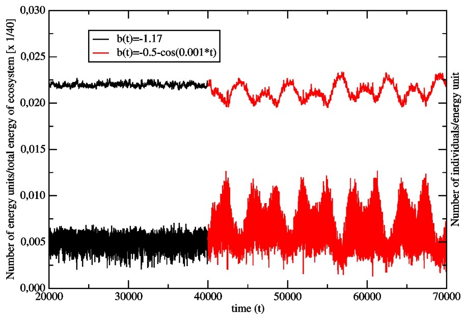
Effect of the transition from the time-independent surrounding (b(t)=−1.17, $t < 40 000$ ) to the one varying in time ( $b (t) = - \frac{1}{2} - \cos (0.001 t)$ , $t ⩾ 40 000$ ) on the size of the single species (a_R=5, a_max=11) and on the number of energy units available for the species. The bottom curve follows the size changes of the species, whereas the upper curve shows the corresponding energy changes in the ecosystem.

In Fig. 3 we have presented the age profiles of the fraction of the inactive ‘chronological’ genes in the population from Fig. 2. The profiles concerning the generations at $t = 20 000$ and $t = 40 000$ refer to a time-independent surrounding. Although we have introduced in the model the back mutations for the inactive genes (the bit-strings corresponding to inactive genes may mutate into another bit-string with probability ρ=0.1), we can observe that, while time is increasing, the shape of the profiles tends to the time-independent one. It determines the average life span of individuals that is ranging between the ages a=1 and a=7. On the other hand, the profiles corresponding to a time-dependent environment show both shrinking and enlarging of the life span. Effectively, the population becomes much younger than during its previous evolution in the time-independent surrounding. More frequent fluctuations of the surrounding make this effect even stronger. This is evident from Fig. 4, where the same old species under consideration experiences the surrounding changing with the higher frequency ω=0.01. We can observe that the effect of the frequently changing environment becomes more destructive for the older members of the species. All our simulation were done with a constant mutation rate (one mutation per genome) and we did not discuss the effect of the various values of the mutation rate on the above results.

Fig. 3
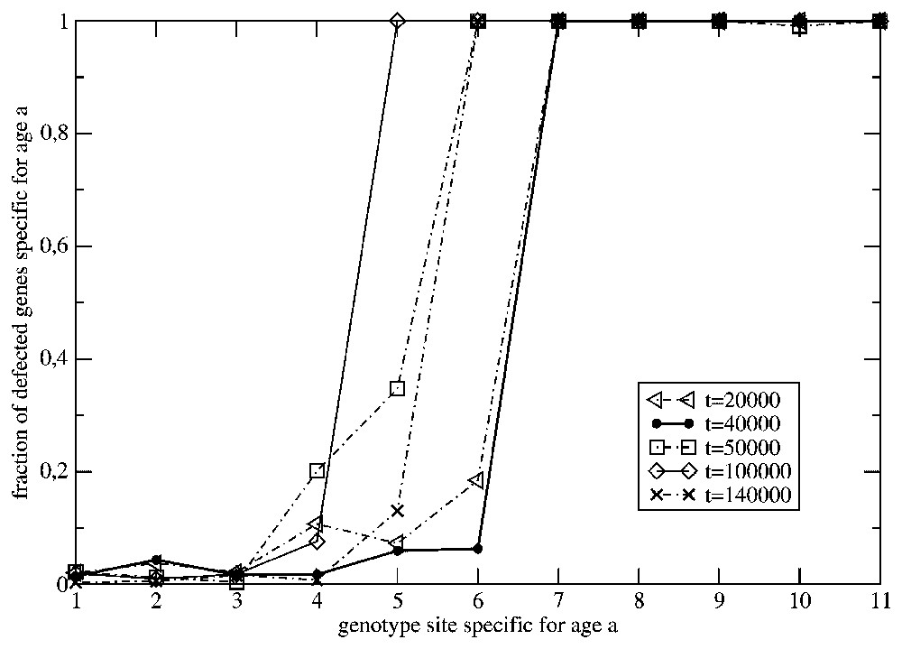
The effect of the change of the time-independent surrounding to the one varying in time, at $t ⩾ 40 000$ , on the distribution of the defected ‘chronological’ genes for the situation presented in Fig. 2.

Fig. 4
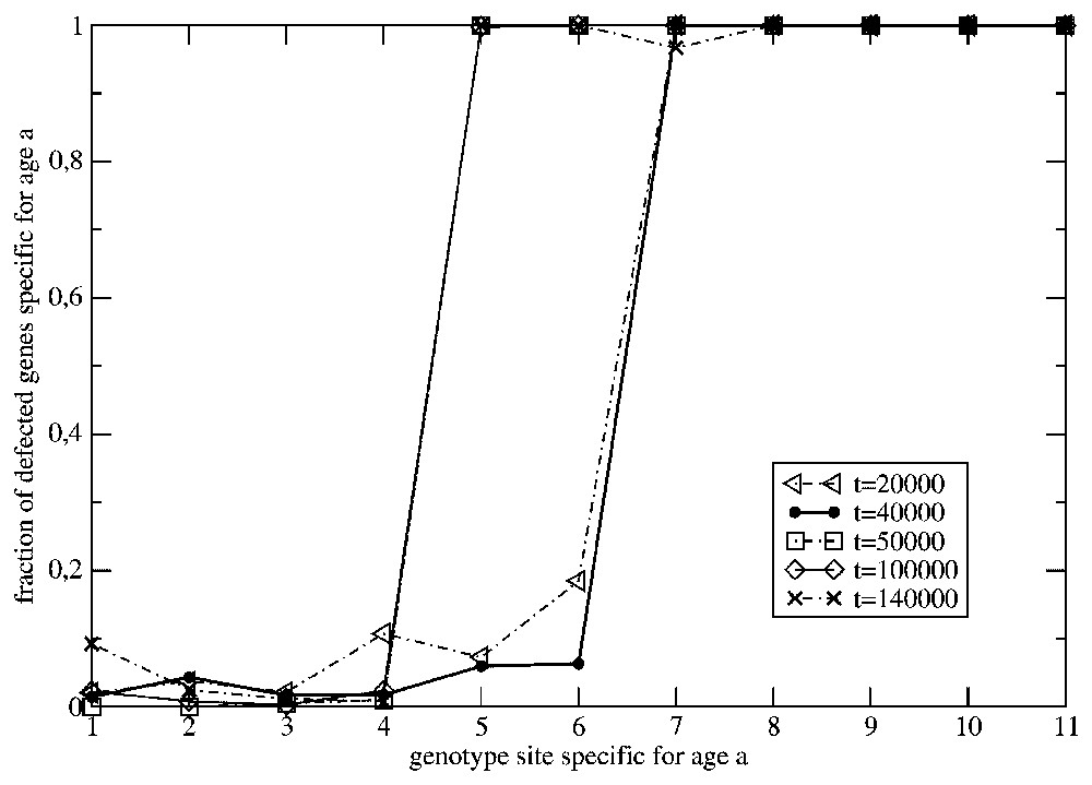
The same as in in Fig. 2, but ω=0.01.

The evolution of the average phenotype of the species from the example in Fig. 2 has been shown in Fig. 5. The same data, but presented with the help of a histogram, have been shown in Fig. 6.

Fig. 5
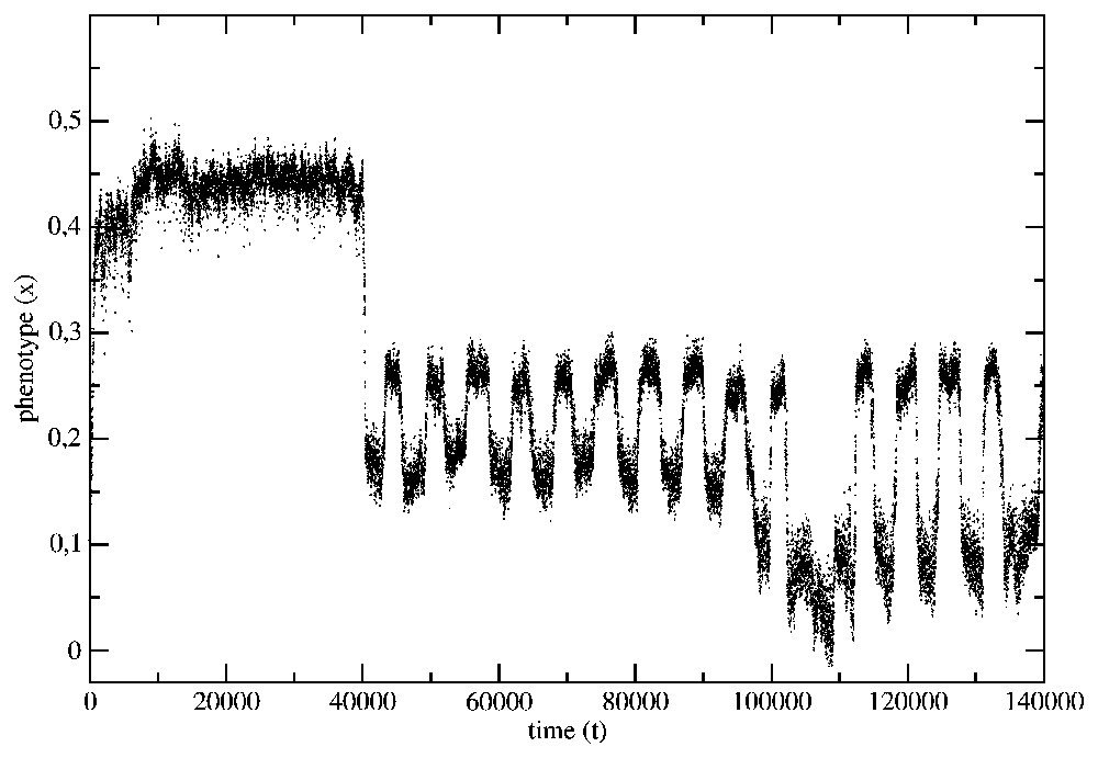
The phenotype evolution for the situation presented in Fig. 2.

Fig. 6
The histogram of the average usage of the phenotype x in the evolving species (from Fig. 2) when there is a time-independent surrounding (r.h.m. histogram), and when there is a fluctuating environment.

Notice that there is a trend to minimize the environment fluctuations and that the genes, which were well adapted in the time-independent environment, do not have the ability to follow the environment fluctuations. They can be even eliminated from the genetic bank of the species if the fluctuations become more frequent.

The environmental changes influence the size of all species in the ecosystem and this is the reason why some of them may be eliminated. The regeneration of the energy resources in the ecosystem takes some time and too rapid a growth of some species, e.g., mutant species, acts as a sudden cataclysm for the other species. The Lotka–Volterra systems have a self-regulatory character and there exist threshold values for the fraction of destroyed population above which the system returns to its previous state [8,18]. However, in the case of genetic populations, if the catastrophe is applied for many generations, one can observe that the age profile of the fraction of defective genes in the population may loose its stability and next the species becomes extincted [8]. Thus the appearance of the new species, even for a relatively short period, can eliminate the old species.

In our computer simulations, we associate a new value, a_R, of the reproduction age with every new species appearing in the course of evolution. The value is determined with the help of a computer random-number generator. Thus, we have also the possibility to investigate the effect of the reproduction age on the adaptation of the species to the fluctuating surrounding. We have observed that the events representing the appearance of the new species with the small value a_R (a_R∼1), are usually represented by short-duration ‘bursts’ of the population size and they vanish as rapidly as they have appeared. In the example in Fig. 7, the are represented by the highest blobs painted in black, at the bottom of the figure. This phenomenon is easy to explain as in this case the life span of individuals is practically shrinking to the activity of single genes and the individuals die after they reproduce themselves. The active genes cannot effectively adapt to the changing environment. How important the range of life span for species stability is, can be also concluded from the histograms in Fig. 8.

Fig. 7
The effect of the speciation from the old species (earlier aging for 40 000 generations in a time-independent environment) in a fluctuating environment ( $b (t) = - \frac{1}{2} - \cos (0.01 t$ ), on the evolution of the energy resources. In the bottom part of the figure, a few examples of the new species created in the course of the evolution have been shown. The energy cost of the new species creation or extinction is reflected by the terrace-like changes in the upper curve. The survived species have not been shown for clarity of the picture.

Fig. 8
Histograms of the phenotype usage in the environment changing with the frequency ω=0.02 in the case of three species: the predecessor population (a_R=5), and two descendant populations (a_R=7, a_R=2). The frequency of the environment changes is ω=0.02.

Histograms of the average usage of the phenotype x of the species representing the predecessor (a_R=5) and two descendant species (a_R=2,7) are presented in Fig. 8. It is evident that the average value x representing the species with a_R=2 oscillates far away from the optimum values (variable minima of V(x,t)), because there is an insufficient number of genes adapted to the variable surrounding. The situation is a little bit better with the predecessor (old species). However, it is evident that it cannot be stable over a long time in a variable surrounding. The most stable species is the one for which a_R=7, because in its population there are inherited genes which have adapted to the variable surrounding (the range of x is almost symmetric with respect to x=0).

In this study, we did not discuss the mechanism of speciation in the new species. We have restricted our analysis to the ‘first-order’ speciation originating from old species and we discussed in detail its effect on the inherited genetic information. We could expect a chain of events representing speciation with the species being better and better adapted to the environment. The younger the species, the more probable speciation, and one should observe peaks in the number of speciation events in a short period.

6 Conclusions

We have discussed a model of species evolution in an ecosystem where the energy resources regenerate themselves according to a logistic differential equation. The number of species present in the ecosystem under consideration results from evolution, which is understoood as the interplay of the two processes only, mutation and selection. We observed that after long periods of ‘stasis’ there are bursts of the new species that are able to live for thousands of generations. We have observed that in a variable surrounding, the species for which the reproduction age a_R is too small are very unstable, even if their size substantially exceeds the specific size for other species. In our model, they usually cause the elimination of other species. Simultaneously, the resulting increase in the energy resources makes the next speciations possible.

There are two approaches to the description of species evolution: the one with continuous evolutionary changes and the theory of punctated equilibrium [19,20], according to which the evolutionary activity occurs in bursts. It is often the case that the mathematical models concerning the species evolution are restricted to pure species dynamics consideration or pure genetics evolution. We have shown that the small changes of the inherited genetic information could be the mechanisms of the abrupt evolutionary changes.

Bibliographie

[1] V. Volterra Théorie mathématique de la lutte pour la vie, Gauthier-Villars, Paris, 1931

[2] L.E. Reichl A Modern Course in Statistical Physics, Arnold, 1980 (pp. 641–644)

[3] R. Gerami; M.R. Ejtehadi A history-dependent stochastic predator–prey model: chaos and its elimination, Eur. Phys. J. B, Volume 13 (2000), pp. 601-606

[4] B.E. Kendall Cycles, chaos, and noise in predator–prey dynamics, Chaos, Solitons and Fractals, Volume 12 (2001), pp. 321-332

[5] V. Rai; W.M. Schaffer Chaos in ecology, Chaos, Solitons and Fractals, Volume 12 (2001), pp. 197-203

[6] J. Vandermeer; L. Stone; B. Blasius Categories of chaos and fractal basin boundaries in forced predator–prey models, Chaos, Solitons and Fractals, Volume 12 (2001), pp. 265-276

[7] A.F. Rozenfeld; E.V. Albano Study of a lattice-gas model for a prey–predator system, Physica A, Volume 266 (1999), pp. 322-329

[8] A. Duda; P. Dyś; A. Nowicka; M.R. Dudek Effect of inherited genetic information on stochastic predator–prey model, Int. J. Mod. Phys. C, Volume 11 (2000), pp. 1527-1538

[9] R.M. May Biological populations with nonoverlapping generations: stable points, stable cycles and chaos, Science, Volume 186 (1974), pp. 645-647

[10] R.M. May Simple mathematical models with very complicated dynamics, Nature, Volume 216 (1976), pp. 459-467

[11] T.S. Ray; L. Moseley; N. Jan A predator–prey model with genetics: transition to a self-organized critical state, Int. J. Mod. Phys. C, Volume 9 (1998), pp. 701-710

[12] T.J.P. Penna A bit-string model for biological aging, J. Stat. Phys., Volume 78 (1995), pp. 1629-1633

[13] S. McManus; D.L. Hunter; N. Jan; T. Ray; L. Moseley Speciation from evolution, Int. J. Mod. Phys. C, Volume 10 (1999), pp. 1295-1302

[14] J.H.E. Cartwright; O. Piro The dynamics of Runge–Kutta methods, Int. J. Bifurc. Chaos, Volume 2 (1992), pp. 427-449

[15] E. Niewczas; A. Kurdziel; S. Cebrat Housekeeping genes and death genes in the Penna aging model, Int. J. Mod. Phys. C, Volume 11 (2000), pp. 775-783

[16] S. Moss de Oliveira; P.M.C. de Oliveira Evolution, Money, War, and Computers, Teubner, Stuttgart, Germany, 1999

[17] S. Cebrat Penna model from the perspective of one geneticist, Physica A, Volume 258 (1998), pp. 493-498

[18] A. Pȩkalski; D. Stauffer Three species Lotka–Volterra model, Int. J. Mod. Phys. C, Volume 9 (1998), pp. 777-784

[19] P. Bak; K. Sneppen Punctated equilibrium and criticality in a simple model of evolution, Phys. Rev. Lett., Volume 71 (1993), pp. 4083-4086

[20] K. Sneppen Extremal dynamics and punctated co-evolution, Physica A, Volume 221 (1995), pp. 168-179

Commentaires - Politique