An <i>in silico</i> target identification using Boolean network attractors: Avoiding pathological phenotypes

Arnaud Poret; Jean-Pierre Boissel

doi:10.1016/j.crvi.2014.10.002

Biological modelling/Biomodélisation

An in silico target identification using Boolean network attractors: Avoiding pathological phenotypes
[Identification in silico de cibles au moyen des attracteurs des réseaux Booléens : éviter les phénotypes pathologiques]

Arnaud Poret ^1,² ; Jean-Pierre Boissel ¹

¹ Novadiscovery, 60, avenue Rockefeller, 69008 Lyon, France
² UMR CNRS 5558, 43, boulevard du 11-Novembre-1918, 69622 Villeurbanne cedex, France

Comptes Rendus. Biologies, Volume 337 (2014) no. 12, pp. 661-678.

Résumés

Anglais
Français

Target identification aims at identifying biomolecules whose function should be therapeutically altered to cure the considered pathology. An algorithm for in silico target identification using Boolean network attractors is proposed. It assumes that attractors correspond to phenotypes produced by the modeled biological network. It identifies target combinations which allow disturbed networks to avoid attractors associated with pathological phenotypes. The algorithm is tested on a Boolean model of the mammalian cell cycle and its applications are illustrated on a Boolean model of Fanconi anemia. Results show that the algorithm returns target combinations able to remove attractors associated with pathological phenotypes and then succeeds in performing the proposed in silico target identification. However, as with any in silico evidence, there is a bridge to cross between theory and practice. Nevertheless, it is expected that the algorithm is of interest for target identification.

L’identification de cibles vise à identifier des biomolécules dont la fonction devrait être altérée pour guérir la pathologie considérée. Un algorithme pour l’identification in silico de cibles au moyen des attracteurs des réseaux booléens est proposé. Il suppose que les attracteurs correspondent aux phénotypes produits par le réseau biologique modélisé. Il identifie des combinaisons de cibles qui permettent aux réseaux perturbés d’éviter les attracteurs associés aux phénotypes pathologiques. L’algorithme est testé sur un modèle booléen du cycle cellulaire, et ses applications sont illustrées sur un modèle booléen de l’anémie de Fanconi. Les résultats montrent que l’algorithme retourne des combinaisons de cibles capables de supprimer les attracteurs associés aux phénotypes pathologiques et donc réussit l’identification in silico de cibles proposée. En revanche, comme tout résultat in silico, il y a un pont à franchir entre théorie et pratique. Cependant, il est escompté que l’algorithme présente un intérêt pour l’identification de cibles.

Métadonnées

Reçu le : 2014-05-14
Accepté le : 2014-10-12
Publié le : 2014-11-11

PMID

DOI : 10.1016/j.crvi.2014.10.002

Keywords: Attractors, Boolean networks, Drug discovery, Fanconi anemia, In silico, Phenotypes, Target identification
Mot clés : Attracteurs, Réseaux booléens, Découverte de médicaments, Anémie de Fanconi, In silico, Phénotypes, Identification de cibles

Affiliations des auteurs :

Arnaud Poret ^{1, 2} ; Jean-Pierre Boissel ¹

¹ Novadiscovery, 60, avenue Rockefeller, 69008 Lyon, France
² UMR CNRS 5558, 43, boulevard du 11-Novembre-1918, 69622 Villeurbanne cedex, France

@article{CRBIOL_2014__337_12_661_0,
     author = {Arnaud Poret and Jean-Pierre Boissel},
     title = {An \protect\emph{in silico} target identification using {Boolean} network attractors: {Avoiding} pathological phenotypes},
     journal = {Comptes Rendus. Biologies},
     pages = {661--678},
     publisher = {Elsevier},
     volume = {337},
     number = {12},
     year = {2014},
     doi = {10.1016/j.crvi.2014.10.002},
     language = {en},
}

TY  - JOUR
AU  - Arnaud Poret
AU  - Jean-Pierre Boissel
TI  - An in silico target identification using Boolean network attractors: Avoiding pathological phenotypes
JO  - Comptes Rendus. Biologies
PY  - 2014
SP  - 661
EP  - 678
VL  - 337
IS  - 12
PB  - Elsevier
DO  - 10.1016/j.crvi.2014.10.002
LA  - en
ID  - CRBIOL_2014__337_12_661_0
ER  -

%0 Journal Article
%A Arnaud Poret
%A Jean-Pierre Boissel
%T An in silico target identification using Boolean network attractors: Avoiding pathological phenotypes
%J Comptes Rendus. Biologies
%D 2014
%P 661-678
%V 337
%N 12
%I Elsevier
%R 10.1016/j.crvi.2014.10.002
%G en
%F CRBIOL_2014__337_12_661_0

Arnaud Poret; Jean-Pierre Boissel. An in silico target identification using Boolean network attractors: Avoiding pathological phenotypes. Comptes Rendus. Biologies, Volume 337 (2014) no. 12, pp. 661-678. doi : 10.1016/j.crvi.2014.10.002. https://comptes-rendus.academie-sciences.fr/biologies/articles/10.1016/j.crvi.2014.10.002/

Version originale du texte intégral

1 Introduction

Drug discovery, as its name indicates, aims at discovering new drugs against diseases. This process can be segmented into three steps: i) disease model provision, where experimental models are developed, ii) target identification, where therapeutic targets are proposed, and iii) target validation, where the proposed therapeutic targets are assessed. The present work focuses on the second step of drug discovery: target identification [1,2].

Given an organism suffering from a disease, target identification aims at finding where to act among its multitude of biomolecules in order to alleviate, or ultimately cure, the physiological consequences of the disease. These biomolecules on which perturbations should be applied are called targets and are targeted by drugs [3]. This raises two questions: which target should be therapeutically perturbed and what type of perturbation should be applied. Broadly, the functional perturbation of a target by a drug can be either activating or inactivating, regardless the way the drug achieves it.

One solution is to test all, or at least a large number of, biomolecules for activation or inactivation. Knowing that targeting several biomolecules is potentially more effective [4], the number of possibilities is consequently huge. This rather brute-force screening can be refined with knowledge about the pathophysiology by identifying potential targets based on the role they play in it [5]. Even with this knowledge, experimentally assessing the selected potential targets in vitro or in vivo is far from straightforward. Such experiments are costly in time and resources and exhibit a high risk of failure [6]. Fortunately, in silico experiments appear as valuable tools in improving the efficiency of therapeutic research [7] since they are less costly in time and resources than the traditional in vitro and in vivo ones. However, the stumbling block of in silico experiments is that they are built from the available knowledge: not all is known about everything.

Nevertheless, an impressive and ever increasing amount of biological knowledge is already available in the scientific literature, databases and knowledge bases such as, to name a few, DrugBank [8], KEGG [9], PharmGKB [10], Reactome [11] and TTD [12]. In addition to the complexity of integrating an increasing body of knowledge comes the inherent complexity of biological systems themselves [13]: this is where computational tools can help [14]. The interplay between experimental and computational biology is synergistic rather than competitive [15]. Since in vitro and in vivo experiments produce factual results, they are trustworthy sources of knowledge. Once these factual pieces of knowledge are obtained, computational tools can help to integrate them and infer new ones. This computationally obtained knowledge can be subsequently used to direct further in vitro or in vivo experiments, hence mutually potentiating the whole.

The goal of the present work is to propose a computational methodology implemented in an algorithm for target identification using Boolean network attractors. It assumes that Boolean network attractors correspond to phenotypes produced by the modeled biological network, an assumption successfully applied in several works [16–21] to cite a few. Assuming that a phenotype is an observable and hence a relatively stable state of a biological system and assuming that the state of a biological system results from its dynamics, a phenotype is likely to correspond to an attractor. This assumption can be stated for any dynamical model but, in the present work, only Boolean networks are considered. Reasons are that, in their most basic form, Boolean networks do not require parameter values [22] and that parameter values are not straightforward to estimate due to experimental limitations, particularly at the subcellular scale, the scale where drugs interact with their targets. Moreover, since synchronous Boolean networks are easier to compute than asynchronous ones [23], only synchronous Boolean networks are considered. This does not exclude the possibility, at a later stage, to extend the algorithm for both synchronous and asynchronous updating schemes.

For a biological network involved in a disease, two possible variants are considered: the physiological variant, exhibited by healthy organisms, which produces physiological phenotypes, and the pathological variant, exhibited by ill organisms, which produces pathological phenotypes or which fails to produce physiological ones. A physiological phenotype does not impair life quantity/quality while a pathological phenotype does. It should be noted that the loss of a physiological phenotype is also a pathological condition. The physiological and pathological variants differ in that the latter results from the occurrence of some alterations known to be responsible for disorders. With a pathological variant, there are two non-exclusive pathological scenarios: pathological phenotypes are gained or physiological phenotypes are lost.

The primary goal of the proposed algorithm is to identify, in a pathological variant, target combinations together with the perturbations to apply on them, here called bullets, which render it unable to exhibit pathological phenotypes. The secondary goal is to classify the obtained bullets according to their ability at rendering the pathological variant able to exhibit previously lost physiological phenotypes, if any.

2 Methods

This section briefly introduces some basic principles, namely biological networks [24,25] and Boolean networks [26], defines some concepts and then describes the proposed algorithm. An example network to illustrate it plus a case study to illustrate its intended applications are also described. Finally, some details about implementation and code availability are mentioned.

2.1 Basic principles

2.1.1 Biological networks

A network can be seen as a digraph G = (V, E) where $V = {v_{1}, \dots, v_{n}}$ is the set of cardinality n containing exactly all the nodes $v_{i}$ of the network and where $E = {(v_{i, 1}, v_{j, 1}), \dots, (v_{i, m}, v_{j, m})} \subseteq V^{2}$ is the set of cardinality m containing exactly all the edges $(v_{i}, v_{j})$ of the network [27,28]. In practice, nodes represent entities and edges represent binary relations R ⊆ V² involving them: $v_{i} R v_{j}$ . For example, in gene regulatory networks, nodes represent gene products and edges represent gene expression modulations [29].

2.1.2 Boolean networks

A Boolean network is a network where nodes are Boolean variables x_i and where edges (x_i, x_j) represent the binary is input of relation: x_i is input of x_j. Each x_i has b_i∈ 〚 0, n 〛 inputs $x_{i, 1}, \dots, x_{i, b_{i}}$ . The variables which are not inputs of x_i have no direct influence on it. If b_i = 0 then x_i is a parameter and does not depend on other variables. At each iteration k∈ 〚 k₀, k_end 〛 of the simulation, the value x_i(k) ∈ {0, 1} of each x_i is updated to the value x_i(k + 1) using a Boolean function f_i and the values $x_{i, 1} (k), \dots, x_{i, b_{i}} (k)$ of its inputs, as in the following pseudocode:

1	fork∈ 〚 k₀, k_end − 1 〛 do
2	$x_{1} (k + 1) = f_{1} (x_{1, 1} (k), \dots, x_{1, b_{1}} (k))$
3	…
4	$x_{n} (k + 1) = f_{n} (x_{n, 1} (k), \dots, x_{n, b_{n}} (k))$
5	end for

which can be written in a more concise form:

1	fork∈ 〚 k₀, k_end − 1 〛 do
2	x(k + 1) = f(x(k))
3	end for

where f = (f₁,…,f_n) is the Boolean transition function and x = (x₁,…,x_n) is the state vector. In the present work, it is assumed that k₀ = 1. The value x(k) = (x₁(k),…,x_n(k)) ∈ {0, 1}ⁿ of x at k belongs to the state space S = {0, 1}ⁿ which is the set of cardinality 2ⁿ containing exactly all the possible states. If the values of all the x_i are updated simultaneously at each k then the network is synchronous, otherwise it is asynchronous. With synchronous Boolean networks, x(k) has a unique possible successor x(k + 1): synchronous Boolean networks are deterministic.

In the particular case where k = k₀, x(k₀) = x₀ is the initial state and, in deterministic dynamical systems, determines entirely the trajectory $w = (x (k_{0}), \dots, x (k_{end}))$ . Since it is assumed that k₀ = 1, $w$ is a sequence of length k_end resulting from the iterative computation of x(k) from k₀ to k_end. This iterative computation can be seen as the discretization of a time interval: Boolean networks are discrete dynamical systems as they simulate discretely the time course of the state vector.

The set A = {a₁,…,a_p} of cardinality p containing exactly all the attractors a_i is called the attractor set. Due to the determinism of synchronous Boolean networks, all the attractors are cycles. A cycle is a sequence (x₁,…,x_q) of length q such that ∀j ∈ 〚1, q 〛 , x_j+1 = f(x_j) and x_q+1 = x₁: once the system reaches a state x_j belonging to a cycle, it successively visits its states x_j+1,…,x_q, x₁,…,x_j for infinity. In the particular case where q = 1, the cycle is called a point attractor. The set B_i ⊆ S containing exactly all the x ∈ S from which a_i can be reached is called its basin of attraction. With deterministic dynamical systems, the family of sets (B₁,…,B_p) constitutes a partition of S.

2.2 Definitions

Some concepts used in the present work should be formally defined.physiological phenotype

A phenotype which does not impair life quantity/quality of the organism which exhibits it.

pathological phenotype

A phenotype which impairs life quantity/quality of the organism which exhibits it.

variant (of a biological network)

Given a biological network of interest, a variant of it is one of its versions, namely the network plus eventually some modifications. It should be noted that this does not exclude the possibility that a variant can be the network of interest as is.

physiological variant

A variant which produces only physiological phenotypes. It is the biological network of interest as it should be, namely the one of healthy organisms.

pathological variant

A variant which produces at least one pathological phenotype. It is a dysfunctional version of the biological network of interest, namely a version found in ill organisms.

physiological attractor set

The attractor set A_physio of the physiological variant.

pathological attractor set

The attractor set A_patho of the pathological variant.

physiological Boolean transition function

The Boolean transition function f_physio of the physiological variant.

pathological Boolean transition function

The Boolean transition function f_patho of the pathological variant.

run

An iterative computation of x(k) starting from an x₀ until an a_i is reached. It returns $w = (x (k_{0}), \dots, x (k_{end}))$ where k_end depends on when a_i is reached and hence on x₀.

physiological attractor

An a_i such that a_i ∈ A_physio.

pathological attractor

An a_i such that a_i ∉ A_physio.

modality

The functional perturbation moda_i applied on a node $v_{j} \in V$ of the network, either activating (moda_i = 1) or inactivating (moda_i = 0): at each k, moda_i overwrites f_j(x(k)) and hence x_j(k + 1) = moda_i.

target

A node targ_i ∈ V of the network on which a moda_i is applied.

bullet

A couple (c_targ, c_moda) where c_targ = (targ₁,…,targ_r) is a combination without repetition of targ_i and where c_moda = (moda₁,…,moda_r) is an arrangement with repetition of moda_i, r∈ 〚1, n 〛 being the number of targets in the bullet. Here, moda_i is intended to be applied on targ_i.

therapeutic bullet

A bullet which makes A_patho ⊆ A_physio.

silver bullet

A therapeutic bullet which makes A_patho ⊊ A_physio.

golden bullet

A therapeutic bullet which makes A_patho = A_physio.

The assumed link between phenotypes and attractors is the reason why attractors are qualified as either physiological or pathological according to the phenotype they produce. This is also the reason why, in the present work, target identification aims at manipulating attractor sets of pathological variants.

2.3 Steps of the algorithm

The algorithm has two goals: i) finding therapeutic bullets and ii) classifying them as either golden or silver. A therapeutic bullet makes the pathological variant unable at reaching pathological attractors, that is A_patho ⊆ A_physio. If such a bullet is applied on a pathological variant, the organism bearing it no longer exhibits the associated pathological phenotypes. However, a therapeutic bullet does not necessarily preserve/restore the physiological attractors. If a therapeutic bullet preserves/restores the physiological attractors, namely if A_patho = A_physio, then it is a golden one but if A_patho ⊊ A_physio then it is a silver one.

Given a physiological and a pathological variant, that is f_physio and f_patho, the algorithm follows five steps:

1. with f_physio it computes the control attractor set A_physio
2. it generates bullets and, for each of them, it performs the three following steps
3. with f_patho plus the bullet, it computes the variant attractor set A_patho
4. it assesses the therapeutic potential of the bullet by comparing A_physio and A_patho to detect pathological attractors
5. if the bullet is therapeutic then it is classified as either golden or silver by comparing A_physio and A_patho for equality.

These steps can be written in pseudocode as:

1	with f_physio compute A_physio
2	generate bullet _ set
3	forbullet ∈ bullet _ set do
4	with f_patho plus bullet compute A_patho
5	if A_patho ⊆ A_physio then
6	bullet is therapeutic
7	if A_patho = A_physio then
8	bullet is golden
9	else
10	bullet is silver
11	end if
12	end if
13	end for

The algorithm is described step by step but can be found as one block of pseudocode in Appendix A.

2.3.1 Step 1: computing A_physio

First of all, A_physio has to be computed since it is the control and, as such, determines what is pathological. To do so, runs are performed with f_physio and the reached a_i are stored in A_physio. However, x₀ ∈ S and card S increases exponentially with n. Even for reasonable values of n, card S explodes: more than 1 000 000 possible x₀ for n = 20. One solution ensuring that all the a_i are reached is to start a run from each of the possible x₀, that is from each of the x ∈ S. Practically, this is unfeasible for an arbitrary value of n since the required computational resources can be too demanding. For example, assuming that a run requires 1 millisecond and that n = 50, performing a run from each of the 2⁵⁰ x ∈ S requires nearly 36 000 years.

Given that with deterministic dynamical systems (B₁,…,B_p) is a partition of S, a solution is to select a subset D ⊆ S of a reasonable cardinality containing the x₀ to start from. In the present work, D is selected randomly from a uniform distribution. The stumbling block of this solution is that it does not ensure that at least one x₀ per B_i is selected and then does not ensure that all the a_i are reached. This stumbling block holds only if card D < card S.

Again given that synchronous Boolean networks are deterministic, if a run visits a state already visited in a previous run then its destination, that is the reached attractor, is already found. If so, the run can be stopped and the algorithm can jump to the next one. To implement this, previous trajectories are stored in a set H, the history, and at each k the algorithm checks if $\exists w \in H : x (k) \in w$ . If this check is positive then the algorithm jumps to the next run.

Since, with deterministic dynamical systems, attractors are cycles, the algorithm checks at each k if x(k + 1) is an already visited state of the current run, namely if ∃k′ ∈ 〚1, k 〛 : x(k + 1) = x(k′). If this check is positive then a_i = (x(k′),…,x(k)).

This step can be written in pseudocode as:

1	prompt card D
2	card D = min(card D, 2ⁿ)
3	generate D ⊆ S
4	H = {}
5	A_physio = {}
6	forx₀ ∈ D do
7	k = 1
8	x(k) = x₀
9	while true do
10	if $\exists w \in H : x (k) \in w$ then
11	break
12	end if
13	x(k + 1) = f_physio(x(k))
14	if ∃k′ ∈ 〚1, k 〛 : x(k + 1) = x(k′) then
15	A_physio = A_physio ∪ {(x(k′),…,x(k))}
16	break
17	end if
18	k = k + 1
19	end while
20	H = H ∪ {(x(1),…,x(k))}
21	end for
22	returnA_physio
23	do step 2

Line 2 catches the mistake card D > card S.

It should be noted that the purpose of the present work is not to propose an algorithm for finding Boolean network attractors since advanced algorithms for such tasks are already published [30,31]. The purpose is to introduce a methodology exploiting Boolean network attractors for target identification, a methodology which requires de facto these attractors to be found.

2.3.2 Step 2: generating bullets

Bullets are candidate perturbations to apply on the pathological variant to make it unable at reaching pathological attractors and hence unable at producing pathological phenotypes. Generating a bullet requires a choice of targ_i ∈ V and associated moda_i ∈ {0, 1}. In the present work, there is no time sequencing in target engagement nor in modality application. This means that, given a bullet and during a run, all the targ_i are engaged simultaneously and constantly and the moda_i do not change. As a consequence, for a given bullet, choosing the same targ_i more than once is senseless, while it is possible to choose the same moda_i for more than one targ_i. Therefore, a bullet is a combination c_targ without repetition of targ_i together with an arrangement c_moda with repetition of moda_i.

If bullets containing r targets have to be generated then there are n !/(r ! · (n − r) !) possible c_targ and, for each of them, there are 2^r possible c_moda. This raises the same difficulty than with state space explosion since there are (n ! ·2^r)/(r ! · (n − r) !) possible bullets. For example, with n = 50 and r = 3, there are more than 150 000 possible bullets. Knowing that the algorithm, as explained below, computes one attractor set per bullet, the computation time becomes practically unfeasible.

To overcome this barrier, the algorithm asks for r as an interval 〚r_min, r_max〛, asks for a maximum number $\max_{targ}$ of c_targ to generate and asks for a maximum number $\max_{moda}$ of c_moda to test for each c_targ. The algorithm then generates a set C_targ of c_targ with $card C_{targ} \leq \max_{targ}$ by randomly selecting, from a uniform distribution and without repetition, nodes in the network. In the same way, the algorithm generates a set C_moda of c_moda with $card C_{moda} \leq \max_{moda}$ by randomly choosing, from a uniform distribution and with repetition, modalities as either activating (= 1) or inactivating (= 0).

The result is the bullets: per r∈ 〚 r_min, r_max 〛, a C_targ together with a C_moda. As with state space explosion, the stumbling block of this method is that it does not ensure that all the possible c_targ together with all the possible c_moda are tested. This stumbling block holds only if $\max_{targ} < n! / (r! \cdot (n - r)!)$ or $\max_{moda} < 2^{r}$ .

This step can be written in pseudocode as:

1	prompt $r_{\min}, r_{\max}, \max_{targ}, \max_{moda}$
2	r_max = min(r_max, n)
3	golden _ set = {}
4	silver _ set = {}
5	forr∈ 〚 r_min, r_max 〛 do
6	$\max_{targ}^{r} = \min (\max_{targ}, n! / (r! \cdot (n - r)!))$
7	$\max_{moda}^{r} = \min (\max_{moda}, 2^{r})$
8	C_targ = {}
9	C_moda = {}
10	while $card C_{targ} < \max_{targ}^{r}$ do
11	generate c_targ ∉ C_targ
12	C_targ = C_targ ∪ {c_targ}
13	end while
14	while $card C_{moda} < \max_{moda}^{r}$ do
15	generate c_moda ∉ C_moda
16	C_moda = C_moda ∪ {c_moda}
17	end while
18	do steps 3 to 5
19	end for
20	returngolden _ set, silver _ set

Line 2 catches the mistake r > n. Lines 3 and 4 create sets in which therapeutic bullets found in step 4 are classified as either golden or silver in step 5. Lines 6 and 7 catch the mistake where

\max_{targ}

or

\max_{moda}

is greater than its maximum, which depends on r, hence the creation of

\max_{targ}^{r}

and

\max_{moda}^{r}

to preserve the initially supplied value. Lines 11 and 15 ensure that only new c_targ and c_moda are generated.

2.3.3 Step 3: computing A_patho

Having the control attractor set A_physio and a bullet (c_targ, c_moda) ∈ C_targ × C_moda, the algorithm computes the variant attractor set A_patho under the bullet by almost the same way A_physio is computed in step 1. However, f_patho is used instead of f_physio and the bullet is applied: at each k, f_j(x(k)) is overwritten by moda_i ∈ c_moda, that is x_j(k + 1) = moda_i, provided that $v_{j} = {targ}_{i} \in c_{targ}$ .

In order to apply all the generated bullets, the algorithm uses two nested for loops. For each c_targ ∈ C_targ it uses successively all the c_moda ∈ C_moda. For each (c_targ, c_moda), the algorithm computes the corresponding A_patho and does steps 4 and 5.

This step can be written in pseudocode as:

1	forc_targ ∈ C_targ do
2	for c_moda ∈ C_moda do
3	H = {}
4	A_patho = {}
5	for x₀ ∈ D do
6	k = 1
7	x(k) = x₀
8	while true do
9	if $\exists w \in H : x (k) \in w$ then
10	break
11	end if
12	x(k + 1) = f_patho(x(k))
13	for targ_i ∈ c_targ do
14	for $v_{j} \in V$ do
15	if $v_{j} = {targ}_{i}$ then
16	x_j(k + 1) = moda_i
17	end if
18	end for
19	end for
20	if ∃k′ ∈ 〚1, k 〛 : x(k + 1) = x(k′) then
21	A_patho = A_patho ∪ {(x(k′),…,x(k))}
22	break
23	end if
24	k = k + 1
25	end while
26	H = H ∪ {(x(1),…,x(k))}
27	end for
28	do step 4 and 5
29	end for
30	end for

Lines 13–19 are where bullets are applied.

2.3.4 Step 4: identifying therapeutic bullets

To identify therapeutic bullets among the generated ones, for each (c_targ, c_moda) tested in step 3 and once the corresponding A_patho is obtained, the algorithm compares it with A_physio to check if A_patho ⊆ A_physio. This check ensures that, under the bullet, all the pathological attractors are removed and if new attractors appear then they are physiological ones. If this check is positive, then the bullet is therapeutic and the algorithm pursues with step 5.

This step can be written in pseudocode as:

1	ifA_patho ⊆ A_physio then
2	do step 5
3	end if

2.3.5 Step 5: assessing therapeutic bullets

Therapeutic bullets are qualified as either golden or silver according to their ability at making the pathological variant reaching the physiological attractors. All therapeutic bullets, being golden or silver, remove the pathological attractors without creating new ones, that is A_patho ⊆ A_physio. However, this does not imply that therapeutic bullets preserve/restore the physiological attractors. A golden bullet preserves/restores the physiological attractors: A_patho = A_physio while a silver bullet does not: A_patho ⊊ A_physio.

In this setting, golden bullets are perfect therapies while silver bullets are not. However, since precious things are rare and just as gold is rarer than silver, finding golden bullets is less likely than finding silver ones. Indeed, given that more constraints are required for a therapeutic bullet to be a golden one, it is more likely that the found therapeutic bullets are silver ones, except in one case: card A_physio = 1.

Theorem 1

If card A_physio = 1 then all therapeutic bullets are golden.

Proof

(therapeutic bullet) \Rightarrow (A_{patho} \subseteq A_{physio})

(1)

(1) \Rightarrow (A_{patho} \in P (A_{physio}))

(2)

(card A_{physio} = 1) \Rightarrow (A_{physio} = {a})

(3)

(3) \Rightarrow (P (A_{physio}) = {\emptyset, {a}})

(4)

((2) \land (4)) \Rightarrow ((A_{patho} = {a}) \lor (A_{patho} = \emptyset))

(5)

(deterministic dynamical systems) \Rightarrow (A \neq \emptyset)

(6)

(6) \Rightarrow (A_{patho} \neq \emptyset)

(7)

((5) \land (7)) \Rightarrow (A_{patho} = {a})

(8)

((3) \land (8)) \Rightarrow (A_{patho} = A_{physio})

(9)

(9) \Rightarrow (therapeutic bullet is golden)

(10)

□

Practically, in the present setting, an organism bearing a pathological variant treated with a therapeutic bullet no longer exhibits the associated pathological phenotypes. Moreover, if the therapeutic bullet is golden then the organism exhibits the same phenotypes than its healthy counterpart. However, if the therapeutic bullet is silver then the organism fails to exhibit at least one physiological phenotype. With a silver bullet this is a matter of choice: what is the less detrimental between a silver bullet and no therapeutic bullet at all.

This step can be written in pseudocode as:

1	ifA_patho = A_physio then
2	golden _ set = golden _ set ∪ {(c_targ, c_moda)}
3	else
4	silver _ set = silver _ set ∪ {(c_targ, c_moda)}
5	end if

2.4 Example network

To illustrate the algorithm, it is used on a Boolean model of the mammalian cell cycle published by Faure et al. [18]. This model is chosen for several reasons: i) synchronous updating is performed: to date, the algorithm focuses on synchronous Boolean networks, ii) a mammalian biological system is modeled: the closer to human physiology the model is, the better it illustrates the intended applications, iii) the cell cycle is a at the heart of cancer: this gives relevancy to the example network, iv) the network comprises ten nodes: easily computable in face of its state space and v) attractors are already computed: useful to validate the algorithm in finding them.

Below are the Boolean functions of the example network where, for the sake of readability, x_i stands for x_i(k) and x_i+ stands for x_i(k + 1).

\begin{matrix} {CycD}_{+} & = & CycD \\ {Rb}_{+} & = & (\neg CycD \land \neg CycE \land \neg CycA \land \neg CycB) \lor (p 27 \land \neg CycD \land \neg CycB) \\ E 2 F_{+} & = & (\neg Rb \land \neg CycA \land \neg CycB) \lor (p 27 \land \neg Rb \land \neg CycB) \\ {CycE}_{+} & = & E 2 F \land \neg Rb \\ {CycA}_{+} & = & (E 2 F \land \neg Rb \land \neg Cdc 20 \land \neg (Cdh 1 \land UbcH 10)) \lor (CycA \land \neg Rb \land \neg Cdc 20 \land \neg (Cdh 1 \land UbcH 10)) \\ p 27_{+} & = & (\neg CycD \land \neg CycE \land \neg CycA \land \neg CycB) \lor (p 27 \land \neg (CycE \land CycA) \land \neg CycB \land \neg CycD) \\ Cdc 20_{+} & = & CycB \\ Cdh 1_{+} & = & (\neg CycA \land \neg CycB) \lor Cdc 20 \lor (p 27 \land \neg CycB) \\ UbcH 10_{+} & = & \neg Cdh 1 \lor (Cdh 1 \land UbcH 10 \land (Cdc 20 \lor CycA \lor CycB)) \\ {CycB}_{+} & = & \neg Cdc 20 \land \neg Cdh 1 \end{matrix}

A graphical representation of the example network is shown in Fig. 1.

Fig. 1
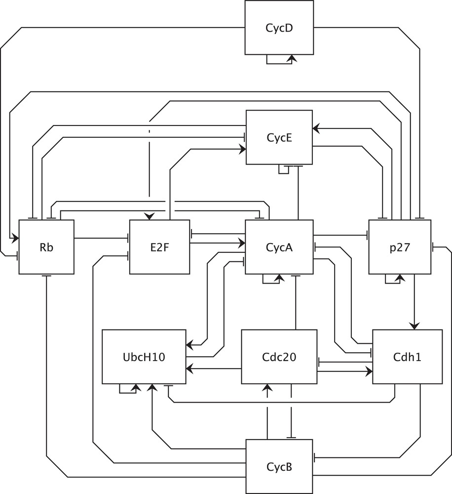
Graphical representation of the example network adapted from [18]. CDKs (cyclin-dependent kinases) are the catalytic partners of cyclins and, in this model, are not explicitly shown since the activity of CDK-cyclin complexes essentially depends on cyclins. Furthermore, inhibition of E2F by Rb is modeled by opposing Rb to the effects of E2F on its targets. The same applies to inhibition of CycE and CycA by p27. For a complete description of the model, please see [18]. CycD: CDK4/6-cyclin D complex, input of the model, initiates the cell cycle, activated by positive signals such as growth factors; CycE: CDK2-cyclin E complex; CycA: CDK2-cyclin A complex; CycB: CDK1-cyclin B complex; Rb: retinoblastoma protein, a tumor suppressor; E2F: a family of transcription factors divided into activator and repressor members, in this model E2F represents activator members; p27: p27/Kip1, a CKI (CDK inhibitor); Cdc20: an APC (Anaphase Promoting Complex, an E3 ubiquitin ligase) activator; Cdh1: an APC activator; UbcH10: an E2 ubiquitin conjugating enzyme.

Having the example network, two variants of it are needed: the physiological one and the pathological one. The physiological variant is the network as is while the pathological variant is the network plus a constitutive activation/inactivation of at least one of its nodes. For simplicity, and given the relatively small number of entities, only one is chosen: the retinoblastoma protein Rb, for which a constitutive inactivation is applied. To implement this, the corresponding f_i becomes:

Rb (k + 1) = 0

in f_patho. Rb is chosen because its inactivation occurs in many cancers [32]. As a consequence, a network bearing a constitutive inactivation of it should be a relevant example of a pathological variant.

2.5 Case study

To illustrate the intended usage of the proposed methodology, the algorithm is used on a Boolean model of the Fanconi Anemia/Breast Cancer (FA/BRCA) pathway published by Rodriguez et al. [33]. This model is chosen for several reasons: i) two pathological conditions are studied: required for a case study of an in silico target identification, ii) the physiological and pathological variants are clearly described: required by the algorithm iii) it is nearly three times bigger than the example network: representative of a more comprehensive biological model while remaining computationally tractable, iv) synchronous updating is used: to date, the algorithm focuses on synchronous Boolean networks and v) attractors are already interpreted in terms of phenotypes.

The FA/BRCA pathway is dedicated to DNA repair and more precisely to interstrand cross-links (ICLs) removal. As expected with any DNA repair impairment, individuals suffering from FA/BRCA pathway malfunction are subjected to increased risk of cancer, such as in Fanconi anemia, a rare genetic disorder causing bone marrow failure, congenital abnormalities and increased risk of cancer [34–36].

Rodriguez et al. propose a Boolean model comprising the FA/BRCA pathway and three types of DNA damages commonly observed in Fanconi anemia, namely ICLs, double-strand breaks (DSBs) and DNA adducts (ADDs). DSBs and ADDs can be created during ICLs repair before being removed, therefore leaving an undamaged DNA ready for the cell cycle. For a complete description of the model, please see [33]. The Boolean functions can be found in Appendix B.

The physiological variant is the FA/BRCA pathway model as is. To it, Rodriguez et al. propose two pathological variants, here called patho1 and patho2, modeling two mutations involving genes of the FA/BRCA pathway. These mutations are observed in patients suffering from Fanconi anemia [37]. The first one involves the FANCA gene, corresponding to the FAcore variable, and the second one involves the FANCD1/BRCA2 or FANCN/PALB2 gene, corresponding to the FANCD1N variable. These mutations are of loss-of-function kind: to simulate them the corresponding f_i becomes

FAcore (k + 1) = 0

for FANCA gene null mutation in f_patho1 and

FANCD 1 N (k + 1) = 0

for FANCD1/BRCA2 or FANCN/PALB2 gene null mutation in f_patho2.

2.6 Implementation

The algorithm is implemented in Fortran 95 compiled with GFortran.¹ The code is available on GitHub² at https://github.com/arnaudporet/kali-targ under a BSD 3-Clause License.³

3 Results

This section exposes results produced with the algorithm on the example network to illustrate how it works. Next, results produced with the algorithm on the case study are exposed to illustrate its intended applications in target identification.

3.1 Results of step 1

Owing to the relatively small size of the example network, card D is set to card S = 1024. Since card D = card S, all the attractors are found. The algorithm returns the following attractors:

a_{1} = \begin{matrix} CycD & 1 & 1 & 1 & 1 & 1 & 1 & 1 \\ Rb & 0 & 0 & 0 & 0 & 0 & 0 & 0 \\ E 2 F & 0 & 1 & 1 & 1 & 0 & 0 & 0 \\ CycE & 0 & 0 & 1 & 1 & 1 & 0 & 0 \\ CycA & 0 & 0 & 0 & 1 & 1 & 1 & 1 \\ p 27 & 0 & 0 & 0 & 0 & 0 & 0 & 0 \\ Cdc 20 & 1 & 0 & 0 & 0 & 0 & 0 & 1 \\ Cdh 1 & 1 & 1 & 1 & 1 & 0 & 0 & 0 \\ UbcH 10 & 1 & 1 & 0 & 0 & 0 & 1 & 1 \\ CycB & 0 & 0 & 0 & 0 & 0 & 1 & 1 \end{matrix} a_{2} = \begin{matrix} CycD & 0 \\ Rb & 1 \\ E 2 F & 0 \\ CycE & 0 \\ CycA & 0 \\ p 27 & 1 \\ Cdc 20 & 0 \\ Cdh 1 & 1 \\ UbcH 10 & 0 \\ CycB & 0 \end{matrix}

each of them attracting 50% of the x ∈ S under f_physio.

Attractors are presented as matrices where, for an attractor of length q, lines correspond to the x_i(k), k∈ 〚1, q 〛 and columns to x(k). A_physio = {a₁, a₂}, which corresponds to results obtained by Faure et al.. By the way, a₁ and a₂ are the two physiological attractors. In terms of phenotypes, a₁ corresponds to the cell cycle while a₂ corresponds to quiescence.

3.2 Results of steps 2 to 5

Results of steps 2 to 5 are grouped since only therapeutic bullets found in step 4 and classified in step 5 are returned. The algorithm is launched with r_min = 1 and r_max = 2. Again due to the relatively small size of the example network, $\max_{targ}$ and $\max_{moda}$ are set to their maximum, namely $\max_{targ} = 45$ and $\max_{moda} = 4$ . As a consequence, all the possible bullets made of 1 to 2 targets are tested. The algorithm returns the following therapeutic bullets:

\begin{matrix} + CycD & silver \\ + CycD & - p 27 & silver \\ - CycD & + Rb & silver \\ + CycD & - Rb & silver \end{matrix}

where + means therapeutic activation and − therapeutic inactivation. It should be noted that no golden bullets are found, an unsurprising result since they are rarer than silver ones. Given these results, the therapeutic activation of Rb alone, which is pathologically inactivated, is not enough to remove the pathological attractors: as seen in the third bullet, the therapeutic activation of Rb must be accompanied by the therapeutic inactivation of CycD.

To better illustrate what is performed to obtain these therapeutic bullets, below is A_patho without any bullet:

a_{3} = \begin{matrix} CycD & 0 & 0 & 0 & 0 & 0 & 0 & 0 & 0 \\ Rb & 0 & 0 & 0 & 0 & 0 & 0 & 0 & 0 \\ E 2 F & 1 & 1 & 1 & 1 & 0 & 0 & 0 & 0 \\ CycE & 0 & 1 & 1 & 1 & 1 & 0 & 0 & 0 \\ CycA & 0 & 0 & 1 & 1 & 1 & 1 & 1 & 0 \\ p 27 & 1 & 1 & 1 & 0 & 0 & 0 & 0 & 0 \\ Cdc 20 & 0 & 0 & 0 & 0 & 0 & 0 & 1 & 1 \\ Cdh 1 & 1 & 1 & 1 & 1 & 0 & 0 & 0 & 1 \\ UbcH 10 & 1 & 0 & 0 & 0 & 0 & 1 & 1 & 1 \\ CycB & 0 & 0 & 0 & 0 & 0 & 1 & 1 & 0 \end{matrix}

a_{4} = \begin{matrix} CycD & 1 & 1 & 1 & 1 & 1 & 1 & 1 \\ Rb & 0 & 0 & 0 & 0 & 0 & 0 & 0 \\ E 2 F & 1 & 1 & 1 & 0 & 0 & 0 & 0 \\ CycE & 0 & 1 & 1 & 1 & 0 & 0 & 0 \\ CycA & 0 & 0 & 1 & 1 & 1 & 1 & 0 \\ p 27 & 0 & 0 & 0 & 0 & 0 & 0 & 0 \\ Cdc 20 & 0 & 0 & 0 & 0 & 0 & 1 & 1 \\ Cdh 1 & 1 & 1 & 1 & 0 & 0 & 0 & 1 \\ UbcH 10 & 1 & 0 & 0 & 0 & 1 & 1 & 1 \\ CycB & 0 & 0 & 0 & 0 & 1 & 1 & 0 \end{matrix}

each of these two attractors attracting 50% of the x ∈ S under f_patho.

It should be noted that a₄ = a₁ ∈ A_physio: a₄ is a physiological attractor. It is possible that the pathological variant produces physiological attractors: A_patho is not the set containing exactly all the pathological attractors, it is the attractor set of the pathological variant. As a consequence, A_physio∩ A_patho ≠ ∅ is possible. However, a₃ ∉ A_physio: it is a pathological attractor and is what a therapeutic bullet, being golden or silver, is intended to avoid.

Again to better illustrate what is performed to obtain these therapeutic bullets, below is A_patho under the third bullet:

\begin{matrix} CycD & 0 \\ Rb & 1 \\ E 2 F & 0 \\ CycE & 0 \\ CycA & 0 \\ p 27 & 1 \\ Cdc 20 & 0 \\ Cdh 1 & 1 \\ UbcH 10 & 0 \\ CycB & 0 \end{matrix}

which is a₂. As expected for a therapeutic bullet, the pathological attractor a₃ is removed. However, the physiological attractor a₁ is not restored: the third bullet is silver. Consequently, with this bullet no cell cycle occurs and the only reachable phenotype is quiescence. While disabling the cell cycle of cancer cells is beneficial, what about disabling the cell cycle of healthy cells. As mentioned above, with silver bullets this is a matter of choice.

3.3 Results on the case study

With the case study, card S = 2²⁸ = 268 435 456: computing attractors from all the x ∈ S becomes too demanding. Indeed, it should be recalled that the algorithm computes one attractor set per bullet, namely A_patho under the tested bullet. As a consequence, card D is set to a more reasonable value: card D = 10 000. Despite that card D < card S, it seems sufficient for the algorithm to find all the attractors, just as Rodriguez et al. whose computation covers the whole state space. Below are the computed attractors:

• A_physio = {a₁}
• A_patho1 = {a₁}
• A_patho2 = {a₁, a₂}, a₁ and a₂ attracting respectively 29.5% and 70.5% of the x ∈ D under f_patho2

and their biological interpretation:

• a₁: cell cycle progression
• a₂: cell cycle arrest

A detailed expression of these attractors can be found in Appendix C.

In physiological conditions, in case of damaged DNA, cells repair it before performing the cell cycle, or die if repair fails. Such checkpoints enable cells to ensure genomic integrity by preventing damaged DNA to be replicated and then propagated [38,39]. Otherwise, genetic instability may appear, potentially leading to cancer [40]. The results show that the physiological variant is able to ensure genomic integrity since its unique attractor is a₁, where ICL = DSB = ADD = 0: DNA damages are repaired, if any, and the cell cycle can safely occur. Interestingly, the same physiological phenotype is computed for patho1 where A_patho1 = A_physio. This suggests that cells bearing FANCA gene null mutation are nonetheless able to repair DNA.

With patho2, a pathological attractor appears: a₂, where DSB = 1. This suggests that cells bearing FANCD1/BRCA2 or FANCN/PALB2 gene null mutation are unable to repair DSBs, explaining why a₂ corresponds to cell cycle arrest: DNA remains damaged. It should be noted that a₁ ∈ A_patho2, suggesting that from certain x₀, that is under certain conditions, such cells could be able to repair DNA. However, a₁ attracts only 29.5% of the x ∈ D under f_patho2, indicating that the pathological phenotype associated with a₂ is more likely to occur.

Altogether, according to computed attractors and their phenotypic interpretation, and limited to the scope studied by the model of Rodriguez et al., FANCA gene null mutation may not induce pathological phenotypes. However, with FANCD1/BRCA2 or FANCN/PALB2 gene null mutation, two phenotypes are predicted: a physiological one and a pathological one, the latter being the most likely to be exhibited. As a consequence, the algorithm has to operate on patho2 to find bullets able to remove the pathological attractor a₂.

By comprehensively testing all bullets made of 1 to 3 targets, the algorithm returns the following results:

	number of all possible bullets	number of therapeutic bullets
r = 1	56	1 (1.786%)
r = 2	1 512	20 (1.323%)
r = 3	26 208	191 (0.729%)

all therapeutic bullets being golden since card A_physio = 1 (see Theorem 1). A list of the computed therapeutic bullets can be found in Appendix D. Given that in a₁, what the pathological variant is forced to reach by means of therapeutic bullets, almost all variables are valued at 0, it is unsurprising that all targets in the computed therapeutic bullets have to be inhibited, that is set to 0.

Occurrence of each node in the found therapeutic bullets, in percentage of the total number of tested bullets, can be found in Appendix E. Below is the top five:

ATM	87.736%
ICL	22.170%
BRCA1	18.396%
DSB	11.792%
MRN	10.377%

In the present case study, DNA damages such as ICLs and DSBs are the pathological events. Unsurprisingly, the algorithm suggests them to be targeted: this is a logical consequence. However, DNA damages are not biomolecules in themselves and directly targeting them by means of drugs appears senseless. What is relevant are the biomolecules of the FA/BRCA pathway suggested as therapeutic targets. Interestingly, ATM dominates all the other candidates, predicting ATM to be a pivotal therapeutic target for the patho2 condition, namely the FA/BRCA pathway bearing FANCD1/BRCA2 or FANCN/PALB2 gene null mutation, as observed in Fanconi anemia.

4 Conclusion

Under the assumption that dynamical system attractors and biological network phenotypes are linked when the former models the latter, the results show that the algorithm succeeds in performing the proposed in silico target identification. It returns therapeutic bullets for a pathological variant of the mammalian cell cycle relevant in diseases such as cancer and for a pathological variant modeling Fanconi anemia. Consequently, the algorithm can be used on other synchronous Boolean models of biological networks involved in diseases for in silico target identification. However, both the physiological and pathological variants have to be known. This can constitute a limit of the proposed methodology since all the pathophysiologies are not known. On the other hand, this can constitute a motivation to unravel pathophysiologies of poorly understood diseases.

Target identification, whether performed in silico or not, is a step belonging to a wider process: drug discovery. Having demonstrated a potential target in silico, or even in vitro, is far from having a drug. Further work and many years are necessary before obtaining a drug which is effective in vivo. For example, and among other characteristics, such a drug has to be absorbed by the organism, has to reach its target and has to be non-toxic at therapeutic dosages. Furthermore, as with any in silico evidence, it should be validated in vitro and ultimately in vivo: there is a bridge to cross between theory and practice. For example, targeting ATM should restore a physiological running of the FA/BRCA pathway bearing FANCD1/BRCA2 or FANCN/PALB2 gene null mutation. However, if ATM operates in other pathways, targeting it may disrupt them, hence creating new pathological conditions. Nevertheless, it is expected that the algorithm is of interest for target identification.

While finding Boolean network attractors of biological networks is not the purpose of the present work, it is a necessary step which is in itself a challenging field of computational biology. As a consequence, incorporating advances made in this field could be a relevant improvement. Another possible improvement could be to extend the algorithm for asynchronous Boolean networks since such models are likely to more accurately describe the dynamics of biological systems. Indeed, in biological systems, events may be subjected to stochasticity, may not occur simultaneously or may not belong to the same time scale, three points that synchronous updating does not take into account. Yet another possible improvement could be to use finer logics, such as multivalued ones. Indeed, one of the main limitations of Boolean models is that their variables can take only two values. In reality, things are not necessarily binary and variables should be able to take more possible values. Multivalued logics enable it in a discrete manner where variables can take a finite number of values between 0 (false) and 1 (true). For example, one can state that Rb is partly impaired rather than totally. Such a statement is not implementable with Boolean models but is with multivalued ones such as, for example, a three-valued logic where true = 1, moderate = 0.5 and false = 0.

Finally, considering basin cardinalities of pathological attractors could be an interesting extension of the proposed criteria for selecting therapeutic bullets. In that case, the therapeutic potential of bullets could be assessed by estimating their ability at reducing the basin of pathological attractors, as performed by Fumia et al. with their Boolean model of cancer pathways [19]. Such a criterion enable to consider the particular case where pathological attractors are removed, that is where pathological basins are reduced to the empty set, but also the other cases where pathological basins are not necessarily reduced to the empty set. Such a less restrictive selection of therapeutic bullets would enable to consider more possibilities for counteracting diseases.

Appendix A

The algorithm in one block of pseudocode.

1	prompt card D
2	card D = min(card D, 2ⁿ)
3	generate D ⊆ S
4	H = {}
5	A_physio = {}
6	forx₀ ∈ D do
7	k = 1
8	x(k) = x₀
9	while true do
10	if $\exists w \in H : x (k) \in w$ then
11	break
12	end if
13	x(k + 1) = f_physio(x(k))
14	if ∃k′ ∈ 〚1, k 〛 : x(k + 1) = x(k′) then
15	A_physio = A_physio ∪ {(x(k′),…,x(k))}
16	break
17	end if
18	k = k + 1
19	end while
20	H = H ∪ {(x(1),…,x(k))}
21	end for
22	return A _physio
23	prompt $r_{\min}, r_{\max}, \max_{targ}, \max_{moda}$
24	r_max = min(r_max, n)
25	golden _ set = {}
26	silver _ set = {}
27	forr∈ 〚 r_min, r_max 〛 do
28	$\max_{targ}^{r} = \min (\max_{targ}, n! / (r! \cdot (n - r)!))$
29	$\max_{moda}^{r} = \min (\max_{moda}, 2^{r})$
30	C_targ = {}
31	C_moda = {}
32	while $card C_{targ} < \max_{targ}^{r}$ do
33	generate c_targ ∉ C_targ
34	C_targ = C_targ ∪ {c_targ}
35	end while
36	while $card C_{moda} < \max_{moda}^{r}$ do
37	generate c_moda ∉ C_moda
38	C_moda = C_moda ∪ {c_moda}
39	end while
40	forc_targ ∈ C_targ do
41	for c_moda ∈ C_moda do
42	H = {}
43	A_patho = {}
44	for x₀ ∈ D do
45	k = 1
46	x(k) = x₀
47	while true do
48	if $\exists w \in H : x (k) \in w$ then
49	break
50	end if
51	x(k + 1) = f_patho(x(k))
52	for targ_i ∈ c_targ do
53	for $v_{j} \in V$ do
54	if $v_{j} = {targ}_{i}$ then
55	x_j(k + 1) = moda_i
56	end if
57	end for
58	end for
59	if ∃k′ ∈ 〚1, k 〛 : x(k + 1) = x(k′) then
60	A_patho = A_patho ∪ {(x(k′),…,x(k))}
61	break
62	end if
63	k = k + 1
64	end while
65	H = H ∪ {(x(1),…,x(k))}
66	end for
67	if A_patho ⊆ A_physio then
68	if A_patho = A_physio then
69	golden _ set = golden _ set ∪ {(c_targ, c_moda)}
70	else
71	silver _ set = silver _ set ∪ {(c_targ, c_moda)}
72	end if
73	end if
74	end for
75	end for
76	end for
77	returngolden _ set, silver _ set

Appendix B

Boolean functions of the case study where, for the sake of readability, x_i stands for x_i(k) and x_i+ stands for x_i(k + 1).

\begin{matrix} {ICL}_{+} & = & ICL \land \neg DSB \\ {FANCM}_{+} & = & ICL \land \neg CHKREC \\ {FAcore}_{+} & = & FANCM \land (ATR \lor ATM) \land \neg CHKREC \\ FANCD 2 I_{+} & = & FAcore \land ((ATM \lor ATR) \lor (H 2 AX \land DSB)) \land \neg USP 1 \\ MUS 81_{+} & = & ICL \\ FANCJBRCA 1_{+} & = & (ICL \lor ssDNARPA) \land (ATM \lor ATR) \\ {XPF}_{+} & = & (MUS 81 \land \neg FANCM) \lor (MUS 81 \land p 53 \land \neg (FAcore \land FANCD 2 I \land FAN 1)) \\ FAN 1_{+} & = & MUS 81 \land FANCD 2 I \\ {ADD}_{+} & = & (ADD \lor (MUS 81 \land (FAN 1 \lor XPF))) \land \neg PCNATLS \\ {DSB}_{+} & = & (DSB \lor FAN 1 \lor XPF) \land \neg (NHEJ \lor HRR) \\ {PCNATLS}_{+} & = & (ADD \lor (ADD \land FAcore)) \land \neg (USP 1 \lor FAN 1) \\ {MRN}_{+} & = & DSB \land ATM \land \neg ((KU \land FANCD 2 I) \lor RAD 51 \lor CHKREC) \\ BRCA 1_{+} & = & DSB \land (ATM \lor CHK 2 \lor ATR) \land \neg CHKREC \\ {ssDNARPA}_{+} & = & DSB \land ((FANCD 2 I \land FANCJBRCA 1) \lor MRN) \land \neg (RAD 51 \lor KU) \\ FANCD 1 N_{+} & = & (ssDNARPA \land BRCA 1) \lor (FANCD 2 I \land ssDNARPA) \land \neg CHKREC \\ RAD 51_{+} & = & ssDNARPA \land FANCD 1 N \land \neg CHKREC \\ {HRR}_{+} & = & DSB \land RAD 51 \land FANCD 1 N \land BRCA 1 \land \neg CHKREC \\ USP 1_{+} & = & ((FANCD 1 N \land FANCD 2 I) \lor PCNATLS) \land \neg FANCM \\ {KU}_{+} & = & DSB \land \neg (MRN \lor FANCD 2 I \lor CHKREC) \\ {DNAPK}_{+} & = & (DSB \land KU) \land \neg CHKREC \\ {NHEJ}_{+} & = & (DSB \land DNAPK \land XPF \land \neg ((FANCJBRCA 1 \land ssDNARPA) \lor CHKREC)) \lor ((DSB \land DNAPK \land KU) \land \neg (ATM \land ATR)) \\ {ATR}_{+} & = & (ssDNARPA \lor FANCM \lor ATM) \land \neg CHKREC \\ {ATM}_{+} & = & (ATR \lor DSB) \land \neg CHKREC \\ p 53_{+} & = & (((ATM \land CHK 2) \lor (ATR \land CHK 1)) \lor DNAPK) \land \neg CHKREC \\ CHK 1_{+} & = & (ATM \lor ATR \lor DNAPK) \land \neg CHKREC \\ CHK 2_{+} & = & (ATM \lor ATR \lor DNAPK) \land \neg CHKREC \\ H 2 {AX}_{+} & = & DSB \land (ATM \lor ATR \lor DNAPK) \land \neg CHKREC \\ {CHKREC}_{+} & = & ((PCNATLS \lor NHEJ \lor HRR) \land \neg DSB) \lor ((\neg ADD) \land (\neg ICL) \land (\neg DSB) \land \neg CHKREC) \end{matrix}

Appendix C

Computed attractors for the case study.

a_{1} = \begin{matrix} ICL & 0 & 0 \\ FANCM & 0 & 0 \\ FAcore & 0 & 0 \\ FANCD 2 I & 0 & 0 \\ MUS 81 & 0 & 0 \\ FANCJBRCA 1 & 0 & 0 \\ XPF & 0 & 0 \\ FAN 1 & 0 & 0 \\ ADD & 0 & 0 \\ DSB & 0 & 0 \\ PCNATLS & 0 & 0 \\ MRN & 0 & 0 \\ BRCA 1 & 0 & 0 \\ ssDNARPA & 0 & 0 \\ FANCD 1 N & 0 & 0 \\ RAD 51 & 0 & 0 \\ HRR & 0 & 0 \\ USP 1 & 0 & 0 \\ KU & 0 & 0 \\ DNAPK & 0 & 0 \\ NHEJ & 0 & 0 \\ ATR & 0 & 0 \\ ATM & 0 & 0 \\ p 53 & 0 & 0 \\ CHK 1 & 0 & 0 \\ CHK 2 & 0 & 0 \\ H 2 AX & 0 & 0 \\ CHKREC & 0 & 1 \end{matrix} a_{2} = \begin{matrix} ICL & 0 \\ FANCM & 0 \\ FAcore & 0 \\ FANCD 2 I & 0 \\ MUS 81 & 0 \\ FANCJBRCA 1 & 1 \\ XPF & 0 \\ FAN 1 & 0 \\ ADD & 0 \\ DSB & 1 \\ PCNATLS & 0 \\ MRN & 1 \\ BRCA 1 & 1 \\ ssDNARPA & 1 \\ FANCD 1 N & 0 \\ RAD 51 & 0 \\ HRR & 0 \\ USP 1 & 0 \\ KU & 0 \\ DNAPK & 0 \\ NHEJ & 0 \\ ATR & 1 \\ ATM & 1 \\ p 53 & 1 \\ CHK 1 & 1 \\ CHK 2 & 1 \\ H 2 AX & 1 \\ CHKREC & 0 \end{matrix}

Appendix D

Therapeutic bullets found for the case study.

−ATM			golden
−ATM	−CHK2		golden
−HRR	−ATM		golden
−ssDNARPA	−ATM		golden
−BRCA1	−ATM		golden
−MRN	−ATM		golden
−FAN1	−ATM		golden
−ICL	−DSB		golden
−FAcore	−ATM		golden
−USP1	−ATM		golden
−ATM	−H2AX		golden
−ADD	−ATM		golden
−RAD51	−ATM		golden
−XPF	−ATM		golden
−FANCM	−ATM		golden
−FANCD1N	−ATM		golden
−ATM	−CHK1		golden
−ICL	−ATM		golden
−ATM	−p53		golden
−FANCJBRCA1	−ATM		golden
−FANCD2I	−ATM		golden
−ICL	−FANCD1N	−ATM	golden
−ICL	−FAcore	−DSB	golden
−BRCA1	−USP1	−ATM	golden
−BRCA1	−ssDNARPA	−ATM	golden
−BRCA1	−ATM	−CHK1	golden
−ADD	−ATM	−H2AX	golden
−FAN1	−MRN	−ATM	golden
−ATM	−CHK2	−H2AX	golden
−ICL	−DSB	−MRN	golden
−XPF	−MRN	−ATM	golden
−FAcore	−FANCD2I	−ATM	golden
−FANCM	−ATM	−CHK2	golden
−RAD51	−ATM	−p53	golden
−ICL	−ssDNARPA	−ATM	golden
−FANCM	−ATR	−ATM	golden
−RAD51	−ATM	−H2AX	golden
−ADD	−FANCD1N	−ATM	golden
−ICL	−USP1	−ATM	golden
−FANCM	−MRN	−ATR	golden
−MRN	−USP1	−ATM	golden
−FAN1	−HRR	−ATM	golden
−BRCA1	−ATM	−H2AX	golden
−FANCJBRCA1	−ADD	−ATM	golden
−MRN	−ssDNARPA	−ATM	golden
−FAcore	−ssDNARPA	−ATM	golden
−FAcore	−FANCD1N	−ATM	golden
−FANCD2I	−BRCA1	−ATM	golden
−ADD	−MRN	−ATM	golden
−ATM	−p53	−CHK2	golden
−RAD51	−ATM	−CHK2	golden
−FANCM	−ATM	−H2AX	golden
−ADD	−PCNATLS	−ATM	golden
−FANCJBRCA1	−ATM	−p53	golden
−FANCM	−MRN	−ATM	golden
−FANCJBRCA1	−ATM	−CHK2	golden
−FANCD2I	−USP1	−ATM	golden
−ADD	−ATM	−CHK2	golden
−FANCD2I	−FANCD1N	−ATM	golden
−MRN	−HRR	−ATM	golden
−ICL	−DSB	−USP1	golden
−FAN1	−FANCD1N	−ATM	golden
−FAN1	−ATM	−H2AX	golden
−FANCJBRCA1	−FAN1	−ATM	golden
−ssDNARPA	−ATM	−H2AX	golden
−ATM	−CHK1	−CHK2	golden
−ADD	−HRR	−ATM	golden
−ATM	−p53	−CHK1	golden
−FAcore	−ATM	−H2AX	golden
−FANCD2I	−ATM	−CHK2	golden
−FAN1	−RAD51	−ATM	golden
−FANCD2I	−RAD51	−ATM	golden
−FANCJBRCA1	−XPF	−ATM	golden
−ICL	−FANCJBRCA1	−DSB	golden
−ssDNARPA	−HRR	−ATM	golden
−MRN	−BRCA1	−ATM	golden
−FANCM	−FAN1	−ATM	golden
−ssDNARPA	−ATM	−p53	golden
−FAN1	−ATM	−CHK2	golden
−FANCD2I	−ssDNARPA	−ATM	golden
−FANCD2I	−FAN1	−ATM	golden
−XPF	−HRR	−ATM	golden
−FAN1	−BRCA1	−ATM	golden
−ADD	−ATM	−CHK1	golden
−FAcore	−HRR	−ATM	golden
−XPF	−ATM	−CHK1	golden
−ADD	−BRCA1	−ATM	golden
−ICL	−FAN1	−DSB	golden
−ADD	−ATM	−p53	golden
−ICL	−MUS81	−ATM	golden
−FAcore	−RAD51	−ATM	golden
−ATM	−CHK1	−H2AX	golden
−ICL	−MRN	−ATM	golden
−ssDNARPA	−ATM	−CHK2	golden
−XPF	−RAD51	−ATM	golden
−FANCM	−ATM	−CHK1	golden
−ICL	−DSB	−KU	golden
−ICL	−MRN	−ATR	golden
−ssDNARPA	−RAD51	−ATM	golden
−FANCJBRCA1	−ssDNARPA	−ATM	golden
−XPF	−ATM	−p53	golden
−FAcore	−MRN	−ATM	golden
−HRR	−ATM	−H2AX	golden
−HRR	−ATM	−p53	golden
−FANCJBRCA1	−FANCD1N	−ATM	golden
−FANCM	−ADD	−ATM	golden
−FAcore	−ATM	−CHK2	golden
−ICL	−ATM	−CHK1	golden
−MRN	−FANCD1N	−ATM	golden
−ADD	−ssDNARPA	−ATM	golden
−MRN	−RAD51	−ATM	golden
−FANCD1N	−ATM	−p53	golden
−FANCD1N	−RAD51	−ATM	golden
−BRCA1	−ATM	−CHK2	golden
−ADD	−RAD51	−ATM	golden
−ICL	−DSB	−FANCD1N	golden
−ICL	−RAD51	−ATM	golden
−ICL	−ATM	−CHK2	golden
−FANCD1N	−ATM	−H2AX	golden
−MRN	−ATM	−H2AX	golden
−FAcore	−FAN1	−ATM	golden
−ICL	−XPF	−ATM	golden
−FANCD2I	−ADD	−ATM	golden
−FANCD2I	−ATM	−H2AX	golden
−ICL	−ATR	−ATM	golden
−FANCM	−HRR	−ATM	golden
−USP1	−ATM	−H2AX	golden
−ICL	−DSB	−RAD51	golden
−ICL	−ATM	−H2AX	golden
−FANCD1N	−USP1	−ATM	golden
−FANCM	−FANCD2I	−ATM	golden
−FANCD2I	−MRN	−ATM	golden
−FAcore	−ADD	−ATM	golden
−ICL	−FAcore	−ATM	golden
−FANCM	−ssDNARPA	−ATM	golden
−XPF	−ATM	−H2AX	golden
−FAcore	−USP1	−ATM	golden
−HRR	−ATM	−CHK1	golden
−BRCA1	−RAD51	−ATM	golden
−FAN1	−ADD	−ATM	golden
−FANCJBRCA1	−MRN	−ATM	golden
−FANCM	−USP1	−ATM	golden
−FANCJBRCA1	−ATM	−H2AX	golden
−FANCM	−FAcore	−ATM	golden
−HRR	−USP1	−ATM	golden
−ICL	−FANCM	−ATM	golden
−ICL	−DSB	−ssDNARPA	golden
−FAN1	−USP1	−ATM	golden
−FANCM	−FANCJBRCA1	−ATM	golden
−ssDNARPA	−ATM	−CHK1	golden
−FAcore	−FANCJBRCA1	−ATM	golden
−FANCD2I	−HRR	−ATM	golden
−FANCD2I	−FANCJBRCA1	−ATM	golden
−XPF	−ssDNARPA	−ATM	golden
−USP1	−ATM	−CHK1	golden
−ICL	−DSB	−ATM	golden
−ICL	−ADD	−DSB	golden
−USP1	−ATM	−CHK2	golden
−XPF	−BRCA1	−ATM	golden
−RAD51	−ATM	−CHK1	golden
−FANCD1N	−ATM	−CHK2	golden
−RAD51	−HRR	−ATM	golden
−ICL	−ATM	−p53	golden
−ICL	−DSB	−DNAPK	golden
−FANCM	−FANCD1N	−ATM	golden
−BRCA1	−FANCD1N	−ATM	golden
−ICL	−HRR	−ATM	golden
−FANCJBRCA1	−HRR	−ATM	golden
−USP1	−ATM	−p53	golden
−XPF	−ATM	−CHK2	golden
−ICL	−DSB	−CHK2	golden
−ICL	−XPF	−DSB	golden
−ssDNARPA	−FANCD1N	−ATM	golden
−FANCJBRCA1	−RAD51	−ATM	golden
−ICL	−DSB	−ATR	golden
−HRR	−ATM	−CHK2	golden
−ADD	−USP1	−ATM	golden
−FANCM	−RAD51	−ATM	golden
−FANCJBRCA1	−ATM	−CHK1	golden
−FANCM	−ATM	−p53	golden
−XPF	−FANCD1N	−ATM	golden
−FAcore	−BRCA1	−ATM	golden
−ICL	−DSB	−NHEJ	golden
−BRCA1	−ATM	−p53	golden
−BRCA1	−HRR	−ATM	golden
−FANCJBRCA1	−USP1	−ATM	golden
−ssDNARPA	−USP1	−ATM	golden
−ICL	−DSB	−H2AX	golden
−FANCM	−BRCA1	−ATM	golden
−MRN	−ATM	−CHK1	golden
−ICL	−FANCJBRCA1	−ATM	golden
−FANCD1N	−ATM	−CHK1	golden
−ICL	−DSB	−BRCA1	golden
−MRN	−ATM	−CHK2	golden
−FANCJBRCA1	−BRCA1	−ATM	golden
−FAN1	−ssDNARPA	−ATM	golden
−MRN	−ATM	−p53	golden
−FANCD1N	−HRR	−ATM	golden
−ICL	−MUS81	−DSB	golden
−ICL	−DSB	−p53	golden
−XPF	−USP1	−ATM	golden
−XPF	−ADD	−ATM	golden
−ATM	−p53	−H2AX	golden
−ICL	−FANCM	−DSB	golden
−ICL	−DSB	−HRR	golden
−ICL	−BRCA1	−ATM	golden
−RAD51	−USP1	−ATM	golden
−ICL	−FAN1	−ATM	golden
−ICL	−ADD	−ATM	golden
−ICL	−DSB	−CHK1	golden
−ICL	−FANCD2I	−DSB	golden
−ICL	−FANCD2I	−ATM	golden

Appendix E

Occurrence of each node in the found therapeutic bullets, in percentage of the total number of tested bullets.

ATM	87.736%
ICL	22.170%
BRCA1	18.396%
DSB	11.792%
MRN	10.377%
FANCM	9.906%
ADD	9.906%
FANCJBRCA1	9.434%
ssDNARPA	9.434%
FANCD1N	9.434%
RAD51	9.434%
HRR	9.434%
USP1	9.434%
CHK2	9.434%
H2AX	9.434%
FAcore	8.019%
FANCD2I	8.019%
FAN1	8.019%
p53	8.019%
CHK1	8.019%
XPF	7.547%
ATR	2.358%
MUS81	0.943%
PCNATLS	0.472%
KU	0.472%
DNAPK	0.472%
NHEJ	0.472%
CHKREC	0%

¹ https://www.gnu.org/software/gcc/fortran/

² https://github.com/

³ https://raw.githubusercontent.com/arnaudporet/kali-targ/master/BSD_3-Clause

Bibliographie

[1] M.A. Lindsay Target discovery, Nat. Rev. Drug Discov., Volume 2 (2003) no. 10, pp. 831-838

[2] J. Knowles; G. Gromo Target selection in drug discovery, Nat. Rev. Drug Discov., Volume 2 (2003) no. 1, pp. 63-69

[3] P. Imming; C. Sinning; A. Meyer Drugs, their targets and the nature and number of drug targets, Nat. Rev. Drug Discov., Volume 5 (2006) no. 10, pp. 821-834

[4] G.R. Zimmermann; J. Lehar; C.T. Keith Multi-target therapeutics: when the whole is greater than the sum of the parts, Drug Discov. Today, Volume 12 (2007) no. 1, pp. 34-42

[5] J.B. Gibbs Mechanism-based target identification and drug discovery in cancer research, Science, Volume 287 (2000) no. 5460, pp. 1969-1973

[6] K. Kaitin Deconstructing the drug development process: the new face of innovation, Clin. Pharmacol. Ther., Volume 87 (2010) no. 3, p. 356

[7] D. Noble; J. Levin; W. Scott Biological simulations in drug discovery, Drug Discov. Today, Volume 4 (1999) no. 1, pp. 10-16

[8] D.S. Wishart; C. Knox; A.C. Guo; D. Cheng; S. Shrivastava; D. Tzur; B. Gautam; M. Hassanali Drugbank: a knowledgebase for drugs, drug actions and drug targets, Nucleic Acids Res., Volume 36 (2008) no. suppl 1, p. D901-D906

[9] M. Kanehisa; S. Goto Kegg: kyoto encyclopedia of genes and genomes, Nucleic Acids Res., Volume 28 (2000) no. 1, pp. 27-30

[10] M. Whirl-Carrillo; E. McDonagh; J. Hebert; L. Gong; K. Sangkuhl; C. Thorn; R. Altman; T.E. Klein Pharmacogenomics knowledge for personalized medicine, Clinical Pharmacol. Ther., Volume 92 (2012) no. 4, pp. 414-417

[11] D. Croft; G. O’Kelly; G. Wu; R. Haw; M. Gillespie; L. Matthews; M. Caudy; P. Garapati; G. Gopinath; B. Jassal et al. Reactome: a database of reactions, pathways and biological processes, Nucleic Acids Res., Volume 39 (2011), p. D691-D697

[12] X. Chen; Z.L. Ji; Y.Z. Chen Ttd: therapeutic target database, Nucleic Acids Res., Volume 30 (2002) no. 1, pp. 412-415

[13] H. Kitano Systems biology: a brief overview, Science, Volume 295 (2002) no. 5560, pp. 1662-1664

[14] H. Kitano Computational systems biology, Nature, Volume 420 (2002) no. 6912, pp. 206-210

[15] B. Di Ventura; C. Lemerle; K. Michalodimitrakis; L. Serrano From in vivo to in silico biology and back, Nature, Volume 443 (2006) no. 7111, pp. 527-533

[16] S. Huang; D.E. Ingber Shape-dependent control of cell growth, differentiation, and apoptosis: switching between attractors in cell regulatory networks, Exp. Cell Res., Volume 261 (2000) no. 1, pp. 91-103

[17] M.I. Davidich; S. Bornholdt Boolean network model predicts cell cycle sequence of fission yeast, PLOS ONE, Volume 3 (2008) no. 2, p. e1672

[18] A. Fauré; A. Naldi; C. Chaouiya; D. Thieffry Dynamical analysis of a generic boolean model for the control of the mammalian cell cycle, Bioinformatics, Volume 22 (2006) no. 14, p. e124-e131

[19] H.F. Fumiã; M.L. Martins Boolean network model for cancer pathways: predicting carcinogenesis and targeted therapy outcomes, PLOS ONE, Volume 8 (2013) no. 7, p. e69008

[20] P. Creixell; E.M. Schoof; J.T. Erler; R. Linding Navigating cancer network attractors for tumor-specific therapy, Nat. Biotechnol., Volume 30 (2012) no. 9, pp. 842-848

[21] K. Baverstock A comparison of two cell regulatory models entailing high dimensional attractors representing phenotype, Progr. Biophys. Mol. Biol., Volume 106 (2011) no. 2, pp. 443-449

[22] M.L. Wynn; N. Consul; S.D. Merajver; S. Schnell Logic-based models in systems biology: a predictive and parameter-free network analysis method, Integr. Biol., Volume 4 (2012) no. 11, pp. 1323-1337

[23] A. Garg; A. Di Cara; I. Xenarios; L. Mendoza; G. De Micheli Synchronous versus asynchronous modeling of gene regulatory networks, Bioinformatics, Volume 24 (2008) no. 17, pp. 1917-1925

[24] X. Zhu; M. Gerstein; M. Snyder Getting connected: analysis and principles of biological networks, Genes Dev., Volume 21 (2007) no. 9, pp. 1010-1024

[25] A.-L. Barabasi; Z.N. Oltvai Network biology: understanding the cell's functional organization, Nat. Rev. Genet., Volume 5 (2004) no. 2, pp. 101-113

[26] S. Bornholdt Boolean network models of cellular regulation: prospects and limitations, J. R. Soc. Interface, Volume 5 (2008) no. Suppl. 1, p. S85-S94

[27] W. Huber; V.J. Carey; L. Long; S. Falcon; R. Gentleman Graphs in molecular biology, BMC Bioinformatics, Volume 8 (2007) no. Suppl 6, p. S8

[28] I.N. Bronshtein; K.A. Semendyayev; G. Musiol; H. Muehlig, Handbook of Mathematics, Springer (2007), pp. 348-359 (Ch. 5)

[29] Y. Xiao A tutorial on analysis and simulation of boolean gene regulatory network models, Curr. Genomics, Volume 10 (2009) no. 7, p. 511

[30] D. Zheng; G. Yang; X. Li; Z. Wang; W. Hung An efficient algorithm for finding attractors in synchronous boolean networks with biochemical applications, Genet. Mol. Res., Volume 12 (2013) no. 4, p. 4656

[31] E. Dubrova; M. Teslenko A sat-based algorithm for finding attractors in synchronous boolean networks, IEEE/ACM Trans. Comput. Biol. Bioinform. (TCBB), Volume 8 (2011) no. 5, pp. 1393-1399

[32] C.J. Sherr; F. McCormick The rb and p53 pathways in cancer, Cancer Cell, Volume 2 (2002) no. 2, pp. 103-112

[33] A. Rodríguez; D. Sosa; L. Torres; B. Molina; S. Frías; L. Mendoza A boolean network model of the fa/brca pathway, Bioinformatics, Volume 28 (2012) no. 6, pp. 858-866

[34] J.P. de Winter; H. Joenje The genetic and molecular basis of fanconi anemia, Mut. Res. Fund. Mol. M., Volume 668 (2009) no. 1, pp. 11-19

[35] A.D. Auerbach Fanconi anemia and its diagnosis, Mut. Res. Fund. Mol. M., Volume 668 (2009) no. 1, pp. 4-10

[36] R.S. Schwartz; A.D. D’Andrea Susceptibility pathways in fanconi's anemia and breast cancer, New Engl. J. Med., Volume 362 (2010) no. 20, pp. 1909-1919

[37] K. Neveling; D. Endt; H. Hoehn; D. Schindler Genotype-phenotype correlations in fanconi anemia, Mut. Res. Fund. Mol. M., Volume 668 (2009) no. 1, pp. 73-91

[38] J. Bartek; J. Lukas Dna damage checkpoints: from initiation to recovery or adaptation, Current opinion in cell biology, Volume 19 (2007) no. 2, pp. 238-245

[39] K. Ishikawa; H. Ishii; T. Saito Dna damage-dependent cell cycle checkpoints and genomic stability, DNA Cell Biol., Volume 25 (2006) no. 7, pp. 406-411

[40] M. Nakanishi; M. Shimada; H. Niida Genetic instability in cancer cells by impaired cell cycle checkpoints, Cancer Sci., Volume 97 (2006) no. 10, pp. 984-989

Commentaires - Politique

1 Introduction

2 Methods

2.1 Basic principles

2.1.1 Biological networks

2.1.2 Boolean networks

2.2 Definitions

2.3 Steps of the algorithm

2.3.1 Step 1: computing Aphysio

2.3.2 Step 2: generating bullets

2.3.3 Step 3: computing Apatho

2.3.4 Step 4: identifying therapeutic bullets

2.3.5 Step 5: assessing therapeutic bullets

Theorem 1

Proof

2.4 Example network

2.5 Case study

2.6 Implementation

3 Results

3.1 Results of step 1

3.2 Results of steps 2 to 5

3.3 Results on the case study

4 Conclusion

Appendix A

Appendix B

Appendix C

Appendix D

Appendix E

2.3.1 Step 1: computing A_physio

2.3.3 Step 3: computing A_patho