On proteins, grids, correlations, and docking

Miriam Eisenstein; Ephraim Katchalski-Katzir

doi:10.1016/j.crvi.2004.03.006

On proteins, grids, correlations, and docking

Présenté par : Stuart Edelstein

Miriam Eisenstein ¹ ; Ephraim Katchalski-Katzir ²

¹ Department of Chemical Research Support, The Weizmann Institute of Science, Rehovot 76100, Israel
² Department of Biological Chemistry, The Weizmann Institute of Science, Rehovot 76100, Israel

Comptes Rendus. Biologies, Volume 327 (2004) no. 5, pp. 409-420.

Résumé

The activity of a living cell can be portrayed as a network of interactions involving proteins and nucleic acids that transfer biological information. Intervention in cellular processes requires thorough understanding of the interactions between the molecules, which can be provided by docking techniques. Docking methods attempt to predict the structures of complexes given the structures of the component molecules. We focus hereby on protein–protein docking procedures that employ grid representations of the molecules, and use correlation for searching the solution space and evaluating putative complexes. Geometric surface complementarity is the dominant descriptor in docking. Inclusion of electrostatics often improves the results of geometric docking for soluble proteins, whereas hydrophobic complementarity is more important in construction of oligomers. Using binding-site information in the scan or as a filter helps to identify and up-rank nearly correct solutions.

Métadonnées

Reçu le : 2004-03-09
Accepté le : 2004-03-16
Publié le : 2004-05-01

PMID

DOI : 10.1016/j.crvi.2004.03.006

Mots clés : molecular recognition, interfaces, structure prediction, Fourier transformations, protein–protein interactions

Affiliations des auteurs :

Miriam Eisenstein ¹ ; Ephraim Katchalski-Katzir ²

¹ Department of Chemical Research Support, The Weizmann Institute of Science, Rehovot 76100, Israel
² Department of Biological Chemistry, The Weizmann Institute of Science, Rehovot 76100, Israel

@article{CRBIOL_2004__327_5_409_0,
     author = {Miriam Eisenstein and Ephraim Katchalski-Katzir},
     title = {On proteins, grids, correlations, and docking},
     journal = {Comptes Rendus. Biologies},
     pages = {409--420},
     publisher = {Elsevier},
     volume = {327},
     number = {5},
     year = {2004},
     doi = {10.1016/j.crvi.2004.03.006},
     language = {en},
}

TY  - JOUR
AU  - Miriam Eisenstein
AU  - Ephraim Katchalski-Katzir
TI  - On proteins, grids, correlations, and docking
JO  - Comptes Rendus. Biologies
PY  - 2004
SP  - 409
EP  - 420
VL  - 327
IS  - 5
PB  - Elsevier
DO  - 10.1016/j.crvi.2004.03.006
LA  - en
ID  - CRBIOL_2004__327_5_409_0
ER  -

%0 Journal Article
%A Miriam Eisenstein
%A Ephraim Katchalski-Katzir
%T On proteins, grids, correlations, and docking
%J Comptes Rendus. Biologies
%D 2004
%P 409-420
%V 327
%N 5
%I Elsevier
%R 10.1016/j.crvi.2004.03.006
%G en
%F CRBIOL_2004__327_5_409_0

Miriam Eisenstein; Ephraim Katchalski-Katzir. On proteins, grids, correlations, and docking. Comptes Rendus. Biologies, Volume 327 (2004) no. 5, pp. 409-420. doi : 10.1016/j.crvi.2004.03.006. https://comptes-rendus.academie-sciences.fr/biologies/articles/10.1016/j.crvi.2004.03.006/

Version originale du texte intégral

1 Introduction

Practically every process in the living cell requires molecular recognition and formation of complexes, which may be stable or transient assemblies of two or more molecules with one molecule acting on the other, or promoting intra- and intercellular communication, or permanent oligomeric ensembles. The development of proteomics methods, such as two-hybrid assays, which provide ample information about protein–protein interactions in vivo, has modified our view of the living cell, emphasizing the importance of signaling cascades and networks of interactions. The rapid accumulation of data on protein–protein interactions, sequences, and structures calls for the development of computational methods to process and combine the information. Particularly important are the methods designed to predict structures of molecular complexes and ensembles that cannot be studied by current experimental methods; transient complexes, for example, are often too short-lived for crystallization or NMR spectroscopy. In some cases a theoretical approach is the only available tool, as for example in studies of antibody recognition of the surfaces of crystals of small organic molecules [1,2].

In docking methods, an attempt is made to predict the structures of complexes given the structures of the component molecules. In the most general case, docking procedures identify the binding sites and predict the relative geometries of the interacting molecules and their conformations in the complex. Over the past 30 years many docking approaches have been proposed (see recent reviews by [3–6]). Most of the methods fall into two categories. One uses direct thermodynamic approaches in which the free energy of the complex, described through different approximations of the enthalpy and entropy terms, is minimized (e.g., [7,8]). The other category includes empirical methods that exploit phenomenological data, such as the geometric and chemical complementarity observed in protein–protein complexes. Although at first glance they appear to be completely different, both approaches are based on the thermodynamics of intermolecular interactions, either directly through enthalpy and entropy equations, or indirectly by considering observed manifestations of the thermodynamics of molecular recognition. For example, shape complementarity reflects the extent of van der Waals interactions for a given interface. More importantly, it also provides an estimate of the number of water molecules that are released to the bulk upon complex formation (desolvation), hence of the entropy change. The latter is the driving force for complex formation in aqueous solution at room temperature [9], and therefore geometric complementarity provides a strong measure of the stability of a complex.

Different empirical docking approaches have been described, each one employing a combination of methods for representing the molecules, searching the solution space, and evaluating the quality of the different complexes. For example, approaches that use correlation for searching the solution space and assessing their quality were combined with different grid representations of the molecules (see below), a genetic algorithm was successfully combined with a molecular surface dot representation [10] or with an atomic representation [11], and computer vision techniques for matching the molecules were found to combine well with knob and hole representations [12].

In this review we focus on protein–protein docking procedures that employ various grid representations of the molecules, and use correlations for searching the solution space and evaluating the putative complexes. Notably, these algorithms treat the molecules as rigid bodies, reducing the docking problem to a six-dimensional search through the rotation–translation space. Thus, conformations of the docked molecules are not changed, although some geometric mismatching is tolerated (see below).

2 First steps in protein–protein docking using grid representations

The use of three-dimensional (3D) grids to represent molecules was introduced into molecular docking independently by Jiang and Kim [13] and Katchalski-Katzir et al. [14] at approximately the same time. Although similar, the two docking algorithms differ in several details. Jiang and Kim [13] combine two representations of the molecule: surface dots with attached surface normals as proposed by Connolly [15], and volume (interior) and surface cubes, the latter containing 2–3 surface dots each. The match between the molecular surfaces at each relative position is evaluated by the number of matching dots, requiring that the cubes containing them overlap and that their attached normals point in approximately opposite directions. The approach of Katchalski-Katzir et al. [14] is simpler in two ways. First, only one representation is employed; the molecules are digitized onto 3D grids, and the surface and the interior of the molecule are distinguished from each other by a digital process that does not require calculation of surface dots. Secondly, for each orientation the correlation function is calculated via Fast Fourier Transformations (FFT), thereby implicitly searching through all the relative translations. The grid (or the equivalent cube) representation effectively softens the surfaces of the molecules, allowing some interpenetration.

The simple and straightforward combination of grid representations with rapid matching of the molecular surfaces by calculation of a correlation function via FFT [14] appealed to a wide readership, and many research groups adopted and modified this approach.

3 The geometric FFT docking algorithm

The 3D structures of protein complexes reveal a close geometric and chemical match between those parts of the molecular surfaces that are in contact. Hence, the shape and other physical characteristics of the surfaces largely determine the nature of the specific interaction. Furthermore, in many cases the 3D structures of the components of the complex closely resemble those of the molecules in their uncomplexed state [16]. Geometric matching is therefore likely to play an important part in determining the structure of the complex.

On the basis of the considerations outlined above, Katchalski-Katzir et al. developed their docking algorithm, which initially assessed only geometric surface complementarity [14]. We describe this algorithm (later named MolFit) in some detail, because many subsequent modifications were derived from it.

The first step in MolFit is the production of grid representations of the two protein molecules a and b, derived from their atomic coordinates, as follows:

{\bar{a}}_{l, m, n} = \{\begin{matrix} 1 on the surface of the molecule \\ ρ inside the molecule \\ 0 outside the molecule \end{matrix}\} and

{\bar{b}}_{l, m, n} = \{\begin{matrix} 1 on the surface of the molecule \\ δ inside the molecule \\ 0 outside the molecule \end{matrix}\}

where l, m, and n are indices of the 3D grid of dimension N×N×N; l,m,n=(1,…,N). Any grid point is considered to be part of the molecule (either ‘surface’ or ‘inside’) if there is at least one atomic nucleus within a distance r from it, where r is in the order of the atomic van der Waals radius. However, different values are assigned to grid points within a surface layer of given thickness and to internal grid points. Two-dimensional cross-sections of these functions are shown in Fig. 1.

Fig. 1
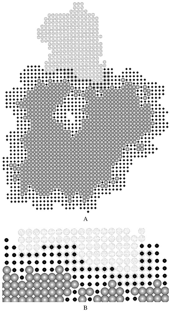
Two-dimensional cross-sections of the grid representations employed by **MolFit** for molecules a and b. The light gray spheres and the small black spheres denote grid points in the interior and in the surface layer of molecule a, respectively. The large dotted spheres denote grid points of molecule b, for which no distinction is made between surface and interior [14]. Molecules a and b are positioned as in the complex, therefore some of the surface grid points of molecule a overlap grid points of molecule b. Such overlaps make positive contributions to the geometric complementarity score. The interface portion of panel A is enlarged in panel B.

Matching of the surfaces is accomplished by calculating the correlation function between the discrete functions $\bar{a}$ and $\bar{b}$ , defined as

{\bar{c}}_{α, β, γ} = \sum_{l = 1}^{N} \sum_{m = 1}^{N} \sum_{n = 1}^{N} {\bar{a}}_{l, m, n} \cdot {\bar{b}}_{l + α, m + β, n + γ}

where α, β, and γ are the numbers of grid steps by which molecule b is shifted with respect to molecule a in each dimension. If the shift vector (α, β, γ) is such that there is no contact between the two molecules, the correlation value is zero. If there is contact between the surfaces, the contribution to the correlation values is positive (see Fig. 1). However, since interpenetration is physically not possible, a distinction between surface contact and penetration must be clearly formulated. This is achieved by assigning a large negative value to ρ in

\bar{a}

and a small positive value to δ in

\bar{b}

. Thus, when the shift vector is such that molecule b penetrates molecule a, multiplication of the negative ρ by the positive δ results in a negative contribution to the overall correlation value. Consequently, the correlation value for each displacement is simply the score of the overlapping surface points corrected by the penalty for penetrations. This value, which reflects the degree of surface complementarity, is referred to hereafter as the ‘score’. Notably, the geometric representation of the molecules in MolFit is not symmetrical. Penetration of either the surface or the interior of molecule b into a is prevented, whereas penetration of the surface of molecule a into the interior of molecule b is allowed, introducing additional ‘softening’ of the surface.

A cross-section of a typical correlation function for a good match is presented in Fig. 2. The coordinates of the prominent peak denote the relative shift of molecule b that yields a good match with molecule a. The width of the peak provides a measure of the relative displacement allowed before matching is lost.

Fig. 2
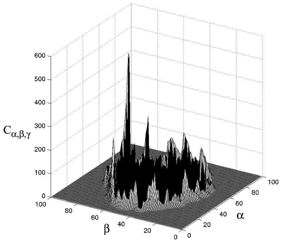
Cross-section of a typical correlation matrix C_α,β,γ. The negative values, which represent positions with sever interpenetration, are denoted by the black area. Note the prominent peak that represents a good match. The coordinates of the peak denote the relative shift of molecule b that yields a good match with molecule a.

Direct calculation of the correlation between the two functions is a rather lengthy procedure, requiring N³ multiplications and additions for each of the N³ possible combinations of α, β, and γ, and resulting in the order of N⁶ computing steps. In contrast, FFT requires the order of N³·ln(N³) steps for transforming a 3D function of N×N×N values.

To complete the general search for a match between the surfaces of molecules a and b, the correlation function $\bar{c}$ has to be calculated for all relative orientations of the molecules. In practice molecule a is stationary, whereas the orientation of the ‘moving’ molecule b is varied at fixed intervals of Δ degrees. For each orientation one or more high-scoring solutions are retained, and at the end of the scan all the solutions are sorted by their scores. The preferred values for the different parameters are summarized in the original paper published by our group [14].

Geometric docking with the MolFit algorithm, as described above, yielded excellent results for the bound docking (defined below) of four protein–protein complexes and one protein–small ligand system, identifying a ‘nearly correct’ solution (defined below) in each case and ranking it very highly (rank 1–5 before refinement and 1 after refinement).

4 Bound versus unbound docking and score versus rank

It is important to clarify the terms often used in determining the success or failure of a docking search. It is common to distinguish between bound docking, i.e. searches that employ the structures of the molecules as they appear in the complex, and unbound docking, in which the structures of one or both molecules are determined separately. In both cases, the accuracy of the predictions is limited by the rigid-body approximation and the discrete translation and rotation grids. We therefore expect that our solutions will be only ‘nearly correct’. The definition of a nearly correct solution differs in different studies that calculate the root mean square difference (RMSD) between (i) Cα atoms of interface residues, (ii) Cα atoms of the whole complex, or (iii) Cα atoms of the ligand molecule (the smaller molecule in the complex; molecule b in the description above) after superposition of the receptor molecule (the larger molecule in the complex; molecule a in the description above). Common criteria are up to 2–2.5 Å RMSD for interface residues, 3–4 Å RMSD for the whole complex, and 7–10 Å RMSD for the ligand molecule.

It is important to ensure that the algorithm not only gives a high score to the nearly correct solution, but that it also distinguishes it from other, false solutions. Therefore, another parameter that reflects the success of a docking search is the rank of the nearly correct solution. This rank, which is the position of the nearly correct solution in the list of solutions sorted by their scores, should be a small number (1 in the optimal case).

5 The first era of FFT docking (bound docking)

The first era of FFT docking was a series of attempts to improve the method of Katchalski-Katzir et al. and make it faster. Vakser and Aflalo [17] used larger grid intervals and considered only complementarity of the hydrophobic portions of the molecular surface by treating the hydrophilic parts as ‘outside the molecule’. They tested the method on four protein–protein complexes and concluded that it yielded better signal-to-noise ratios than geometric docking. Except for the large grid interval, their approach was very similar to the geometric docking of Katchalski-Katzir et al., because they assigned about 80% of the surface as hydrophobic. Meyer et al. [18] replaced the comprehensive search of the rotation–translation space by a partial search, which they limited to conformations capable of forming at least two hydrogen bonds at the interface. They applied the method to 45 complexes using the bound geometries of the molecules, and obtained high-ranking nearly correct predictions (ranking 1–3) in every case. Another procedure that limited the number of relative orientations searched was proposed by Ackermann et al. [19]. Using the FFT procedure, they matched only pre-selected pairs of surface segments. Their scores comprised a geometric complementarity term, a hydrophobic term, and an electrostatic term. Hydrophobicity values and charges were stored in separate sets of grids. The authors applied the method to 51 homo- and heterodimers, employing the bound structures. Despite the elaborate complementarity function, a nearly correct solution (ranking 1–15) with RMSD <3 Å for all Cα atoms was identified for only 18 of the 51 systems. The authors attributed their limited success to the sampling method, and reported that global sampling of the rotation–translation space, using only geometric docking, identified nearly correct solutions ranking 1 for all 51 systems [19].

Several conclusions can be drawn from the results of the abovementioned bound docking studies. First, Katchalski-Katzir et al. and Ackermann et al. obtained very good predictions using only geometric docking. Hence, geometric complementarity appears to be the most dominant term in the evaluation of different docking solutions. Secondly, an exhaustive rotation–translation scan appears to yield better results than partial scans. Thirdly, in all of these studies the docking procedures and parameters were optimized so as to improve the reproduction of known complexes. In unbound docking, however, other parameters might be more appropriate. For example, disassembled complexes were reproduced very well by the procedure of Meyer et al. [18], but the parameters, especially the strict measurements of hydrogen bond geometry, would probably be too limiting in unbound docking.

6 The first docking challenge

Docking programs were first put to the test in the prediction challenge proposed by Strynadka et al. [20]. This was the first blind prediction test, in which the predicting groups submitted their models before the experimental structure of the complex was made available. In such a challenge all participating groups study the same targets, thus eliminating two important factors that make it difficult to compare the performance of different algorithms: choice of targets, which may be harder or easier for prediction, and bias, which is naturally introduced when the predictor knows the expected results.

Six groups participated in the first docking challenge, in which they were required to predict the structure of the complex between TEM1 β-lactamase and the β-lactamase inhibitory protein (BLIP). All six submitted a nearly correct solution, ranked 1, with RMSD values ranging from 1.1 Å (the solution by Eisenstein and Katchalski-Katzir) to 2.5 Å. Very different approaches were used by the participants [20], including energy calculations and estimates of shape complementarity. Janin [21] analyzed the results in terms of the gap between the top ranking (and nearly correct) solution and the next solution. He observed that algorithms that rely on geometric complementarity produced larger gaps than algorithms employing elaborate energy functions. In particular, the electrostatic term was a poor selection criterion. Moreover, algorithms that allowed for conformation changes were not necessarily more successful than the rigid-body docking algorithms.

7 Unbound protein–protein docking

In predicting the structure of the complex between TEM1 β-lactamase and BLIP, the unbound molecular structures were docked. This started a new phase in protein–protein docking, in which the emphasis was on unbound docking. Unbound docking was initially attempted by the two groups that introduced grid representations of molecules into docking [13,14]. Both groups found that their docking algorithms were less successful when unbound structures were used. The inevitable conclusion was that geometric docking fails because structural changes occur upon complex formation. As a next step, additional energy terms (such as electrostatic interactions) were considered in the evaluation of the docking solutions. This was done within the rotation–translation scan or in the context of post-scan re-evaluation filters.

7.1 Electrostatic complementarity

Several attempts were made to introduce electrostatics as an additional term in grid-based docking. Gabb et al. [22] added a test for electrostatic complementarity to the geometric docking method of Katchalski-Katzir et al. The electrostatic descriptor of the stationary molecule was its electrostatic potential, whereas for the moving molecule partial atomic charges were used. The electrostatic descriptors were represented on separate grids and correlated using FFT, producing a Coulombic electrostatic energy term (the product of potential and charge). The electrostatic energy was not added to the geometric complementarity, but was used as a yes/no filter, eliminating docking solutions that were electrostatically unfavorable.

The concept of depicting the electrostatic potential of one molecule and partial atomic charges on the other molecule in additional grids that were distinct from the geometric grids was also employed in the algorithm of Mandell et al. [23]. In that study, however, the potential was described by solvent continuum electrostatics, which captured the effect of the different dielectric constants of the protein and the aqueous solution. In addition, Mandell et al. treated electrostatics as an additional complementarity term, which was combined with the geometric term to produce a composite energy function. Their treatment of geometric complementarity differed from that of Katchalski-Katzir et al., in that they counted the number of intermolecular collisions instead of imposing a grid-based penalty for collisions.

Electrostatic energy was used by Palma et al. as a post-scan filter [24]. These authors calculated the Coulombic energy for the top-ranking solutions from the full scan, but added a dampening constant to the inter-atomic distances to circumvent unrealistic electrostatic repulsion or attraction arising from any small interpenetrations of the docked molecules.

A somewhat different approach was proposed by Heifetz et al. [25]. Instead of calculating the electrostatic energy, which is highly sensitive to structural details and hence to conformation changes, they chose to correlate the electrostatic potentials of the molecules, which reflect their tendency to form good or bad electrostatic interactions. This was based on the previously observed pronounced anti-correlation of the electrostatic potentials at the interface [26]. Heifetz et al. used a single grid of complex numbers to describe each molecule, storing information about the shape of the molecule in the real part and information about its electrostatic character in the imaginary part. Thus,

{\bar{a}}_{l, m, n} = \{\begin{matrix} 1 + i \sqrt{w} E_{a} on the surface of the \\ molecule \\ ρ inside the molecule \\ 0 + i \sqrt{w} E_{a} outside the molecule \end{matrix}\}

and

{\bar{b}}_{l, m, n} = \{\begin{matrix} 1 - i \sqrt{w} E_{b} on the surface and inside \\ the molecule \\ 0 - i \sqrt{w} E_{b} outside the molecule \end{matrix}\}

where

i = \sqrt{- 1}

, E_a and E_b are the electrostatic descriptors for molecules a and b derived from their respective electrostatic potentials, and w is a weight factor determining the relative contributions of the geometric and the electrostatic terms to the complementarity score. The score was equal to the real part of the correlation matrix, depicting the weighted sum of the geometric and electrostatic contributions. It was determined by a single correlation of the grid representations of the complex numbers, using FFT [25].

All of the abovementioned docking procedures have been applied to unbound systems. Some of the studies presented comparisons of geometric and geometric–electrostatic docking results [22,23,25] showing that, in general, inclusion of electrostatic complementarity improved the results of geometric docking. Nevertheless, even in unbound docking, the geometric complementarity term appeared more dominant than the electrostatic term. Heifetz et al. formulated several rules for ‘good electrostatic docking’, which highlighted cases in which inclusion of electrostatic complementarity was likely to improve the geometric docking results.

7.2 Hydrophobic complementarity

Another term employed by several groups in protein–protein docking is desolvation or hydrophobic complementarity. Chen and Weng [27] combined desolvation, geometry, and electrostatics in a multiple-grid representation of each molecule. The desolvation term in that study involved calculation of the correlation between two surfaces weighted by desolvation descriptors (derived from non-pairwise atomic contact energies). This formulation rewarded interfaces with buried aliphatic hydrophobic residues and to lesser extent also those with buried aromatic residues. It reflected the entropic effect resulting from the release of water from the interface, and therefore the desolvation term was intermingled with the geometric term, that represents the same effect. Indeed, when the desolvation term was combined with electrostatics and geometric complementarity, Chen and Weng found that the latter needed to be strongly downscaled.

Berchanski et al., by placing a hydrophobic descriptor in the imaginary part of a grid of complex numbers, formulated a hydrophobic complementarity term that was detached from the geometric term [28]. Their hydrophobic complementarity term rewarded only hydrophobic–hydrophobic contacts, thereby measuring the hydrophobic surface that was packed against the hydrophobic surface of the other molecule. The hydrophobic complementarity score was added to the geometric score. Berchanski et al. found that the effect of hydrophobic complementarity in the docking of soluble proteins was generally small, except for antibody–antigen systems, where up weighting of interactions that involved aromatic residues was beneficial. They also found that intersection of solutions from geometric, geometric–electrostatic, and geometric–hydrophobic docking searches considerably improved the ranking of the nearly correct solutions.

Desolvation energy in a post-scan filter was considered by Jackson et al. [29] and by Palma et al. [24]. Neither group provided information about the effect of desolvation alone. Jackson et al. found that calculation of the desolvation energy, combined with local structure refinement, improved the ranks of nearly correct solutions for enzyme–inhibitor systems but not for antibody–antigen systems.

The different formulations of the hydrophobic effect in the studies described above emphasize the relationship between geometric complementarity and desolvation. Thus, the desolvation term of Chen and Weng [27] incorporates the geometric and the hydrophobic complementarity terms of Berchanski et al. [28]. When separated from the geometric term, hydrophobic complementarity appears to be a weak descriptor in the docking of soluble proteins; its role in the construction of oligomers is more important [28].

7.3 Binding site information

Although inclusion of electrostatic and hydrophobic complementarity terms generally improved the results of unbound docking, as discussed above, it was not enough to rank nearly correct solutions near the top. It was clear that either the dominant geometric complementarity term had to be improved, so that the shape modifications that occur upon complex formation could be more effectively tolerated, or additional information about the interaction site should be included, as is commonly done in protein–ligand docking.

Most of the groups that participated in the first docking challenge used binding-site information as a post-scan filter that eliminated false-positive solutions [20,30]. Several groups [13,22,29,31,32] made such a filter an integral part of their prediction procedure. In contrast, Ben-Zeev and Eisenstein [33] formulated an algorithm to incorporate external information from biological, biochemical, and bioinformatics studies in the scan, generating a different set of solutions, which was biased toward solutions in which several specified residues participated in binding (or did not participate, if this was the preferred option). This was done by storing weights in the imaginary part of a complex numbers grid representation, thus up-weighting or down-weighting given contacts in the geometric scan. The weighted-geometric docking procedure was successfully applied in several cases, using information extracted from bioinformatic analyses [34] or from biochemical studies [35].

Inclusion of binding-site information in the scan or as a filter proved to be a useful tool for identifying and up-ranking nearly correct solutions. Interestingly, Ben-Zeev et al. found that their procedure was successful even when definition of the binding site was approximate, i.e. only part of it was identified and up-weighted, or a portion of the weighted surface was incorrectly assigned [33].

7.4 Different shape descriptors

The dominant role of the geometric complementarity term observed in protein–protein docking suggested that modifying the representation of molecules on the grid was likely to improve the docking results. This was particularly important in the absence of external information. Over the years, different modifications of the original algorithm of Katchalski-Katzir et al. have been proposed. Eisenstein et al. used different radii for different atoms or groups of atoms, with Coulombic radii used to represent oxygen and nitrogen atoms and van der Waals radii for CH_n groups, and modified the molecular surface to represent a solvent-accessible surface [36]. Chen and Weng presented a symmetrical description of the molecular shapes by using grids of complex numbers in which the imaginary part was used to store the interior of the molecule. This approach allowed different penalties to be imposed for surface–interior and interior–interior clashes [27]. The same purpose was achieved by Palma et al. [24] by employing two grids, the surface grid and the interior grid, to describe each molecule. Notably, these authors correlated the grids using Boolean operations, and were therefore able to employ much smaller grids than those used in FFT-based methods.

Several groups proposed different treatments of the outermost atoms of exposed long side chains, such as lysine and arginine, which are also known to be highly flexible. Gabb et al. [22] and Chen and Weng [27] reported that truncating these side chains worsened the docking results for most systems. Palma et al. [24] allowed unrealistic penetration of flexible side chains in their first docking step, and concluded that such softening did not improve the results. A different treatment was proposed by Heifetz and Eisenstein [37], in which the penalty for interpenetration was retained, but contacts formed by the flexible side chains were not rewarded. Their approach led to a significant reduction in the scores of false-positive solutions and improved the rankings of the nearly correct ones.

Another modification of the geometric representation of the molecules was to weight the grid points according to the number of contributing atoms, thereby rewarding positions that allow formation of more intermolecular contacts. Vakser used this approach in conjunction with low-resolution docking [38]. More recently, Chen and Weng weighted only the surface of the stationary molecule, introducing a pairwise shape complementarity descriptor [39] that favored nearly correct solutions, elevating their rankings.

7.5 The CAPRI experiment

The first docking challenge, described above, was a landmark in the development of docking techniques, and stimulated interest in solving the protein–protein docking problem. This initiative was recently continued with the launching of the CAPRI (Critical Assessment of PRediction of Interactions) experiment. CAPRI is an ongoing blind docking experiment [40], which up to now has included 13 targets. The results of this experiment indicate that docking programs often produce good approximate structures of the target complexes [41]. Fig. 3 presents a superposition of the structure of the complex between the basement membrane proteins nidogen and laminin predicted by the group of M. Eisenstein (Eisenstein M., Ben-Zeev E., Atarot T. and Segal D., unpublished results) on the structure obtained experimentally [42]. The binding site is predicted quite accurately (0.8 Å RMSD), providing detailed information on the intermolecular interactions. Notably, despite the rigid-body approximation, the performance of grid-based and other procedures that treat the molecules as rigid bodies was as good as that of non-rigid-body procedures.

Fig. 3
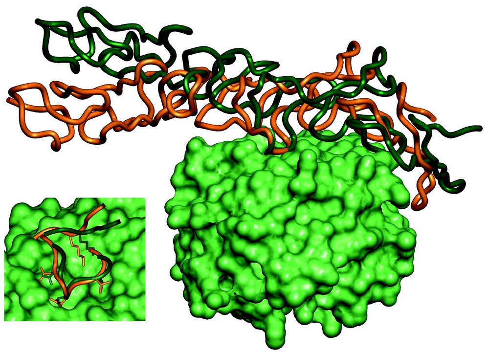
Comparison between the predicted structure of the nidogen–laminin complex, by Eisenstein et al., and the experimental X-ray structure [42]. The nidogen molecules in the predicted and experimental structures were superposed. The surface of nidogen is shown in green. The elongated laminin molecule is shown as a ribbon diagram, orange for the predicted position and dark green for the experimental structure. In the insert we zoom onto the interaction site, showing that despite the deviation between the predicted and observed relative positions of the molecules, most of the binding-site interactions are correctly predicted.

8 Where do we go from here?

The development of docking techniques has progressed significantly over the past few years, starting with bound docking, then proceeding to the far more realistic test of unbound docking, and continuing with blind docking challenges, which provide common ground for comparison of the performance of different docking procedures. Geometric complementarity appears to be an essential feature in complex formation and a powerful descriptor even in unbound docking. Clearly, there is still place for development of new docking techniques and improvement of the old ones. In particular, the approximate solutions provided by most docking programs need to be refined and the question of major conformation changes must be addressed.

The available data on sequence, structure, and intermolecular interaction, as well as our view of the activity in a living cell, are now very different from the situation when docking programs started to emerge, and are likely to change continuously. The development of docking programs will inevitably follow this change. It is likely for example, that many of the structures used for docking will be models at different levels of accuracy, and that docking techniques will evolve to meet this new challenge. Also, new questions will be asked: not only ‘How do molecules a and b bind?’, but also ‘Do molecules a and b bind?’ or ‘Do molecules a, b, c, etc. form an assembly, and if so, how?’ Up to now, model structures have been docked in only a few studies. The low-resolution docking procedure of Vakser et al., which was designed to dock low-accuracy structures [43], has in some cases successfully predicted the structures of complexes starting from very approximate molecular models [44]. Berchanski et al. have succeeded in constructing homo-tetramers from model structures of single subunits by combining molecular modeling with docking [45]. Similarly, only a few attempts have been made to combine more than two domains, subunits, or proteins into assemblies via docking [10,36,45–47], and to our knowledge only one group has attempted to distinguish between true and false protein–protein partners [25].

Docking must also be considered within the larger context of biological sciences. During the past few decades many proteins have been detected in the living cell. Since all of them were located within the relatively small cell volume, an extraordinarily large number of protein–protein interactions could be anticipated. New immunological, genetic, and chemical techniques have been used to identify well-characterized protein complexes in yeast, bacteria, and the fruit fly Drosophila. Some of the proteins were found to interact with only a single partner, whereas others interacted specifically with ensembles of selected proteins. The accumulating information on specific protein–protein interactions led to the construction of maps that clearly showed networks of interactions in the living yeast cells [48–50], bacteria [51] and fruit fly [52].

Most of the interacting proteins in a living cell possess characteristic specific biological activities, which can be arrested or enhanced by interactions with other proteins. Activation of a living cell, either by external stimuli (such as environmental changes or binding of biologically active ligands) or by internal stimuli (such as gene order), is expected to trigger cascades of protein–protein interactions that lead to the desired cellular response. The graphic representation of the flow of information, which is an integral part of protein–protein interaction maps, is expected to uncover such cascades, in which each branch represents a specific signal or information transfer event. Some of the interactions in the cascade may be of extremely short duration, possibly facilitated by an intermolecular contact that does not correspond to the lowest free energy complex. Moreover, during the information transfer some of the proteins within the cell may be destroyed and novel proteins synthesized. Hence, although regular small subsets of interactions have been identified within cellular interaction networks [53], allowing the activity of the cell to be viewed in terms of ‘engineering modules’, the whole cellular network is much more complex than the networks familiar to engineers [54].

We would like to conclude by emphasizing that protein–protein networks exist and transfer biological information using the same factors as those determining protein docking. Any attempt to intervene in cellular processes by changing the information flow within the living cell (e.g., by administration of drugs) requires thorough and detailed understanding of the interactions between the molecules. Such understanding can be provided by docking techniques.

Acknowledgements

We acknowledge the essential contribution of Dr. Isaac Shariv to the development of the MolFit algorithm. MolFit can be downloaded from our web site: http://www.weizmann.ac.il/Chemical_Research_Support/molfit/.

Bibliographie

[1] N. Kessler; D. Perl-Treves; L. Addadi; M. Eisenstein Structural and chemical complementarity between antibodies and the crystal surfaces they recognize, Proteins, Volume 34 (1999), pp. 383-394

[2] M. Geva, M. Eisenstein, L. Addadi, Antibody recognition of chiral surfaces. Structural models of antibody complexes with leucine–leucine–tyrosine crystal surfaces, Proteins, in press

[3] S.J. Wodak; J. Janin Structural basis of macromolecular recognition, Adv. Protein Chem., Volume 61 (2003), pp. 9-73

[4] I. Halperin; B. Ma; H. Wolfson; R. Nussinov Principles of docking: an overview of search algorithms and a guide to scoring functions, Proteins, Volume 47 (2002), pp. 409-443

[5] G.R. Smith; M.J. Sternberg Prediction of protein–protein interactions by docking methods, Curr. Opin. Struct. Biol., Volume 12 (2002), pp. 28-35

[6] M.J. Sternberg; H.A. Gabb; R.M. Jackson Predictive docking of protein–protein and protein–DNA complexes, Curr. Opin. Struct. Biol., Volume 8 (1998), pp. 250-256

[7] J. Fernandez-Recio; M. Totrov; R. Abagyan Soft protein–protein docking in internal coordinates, Protein Sci., Volume 11 (2002), pp. 280-291

[8] J.J. Gray; S. Moughon; C. Wang; O. Schueler-Furman; B. Kuhlman; C.A. Rohl; D. Baker Protein–protein docking with simultaneous optimization of rigid-body displacement and side-chain conformations, J. Mol. Biol., Volume 331 (2003), pp. 281-299

[9] T.E. Creighton Protein Structures and Molecular Properties, Freeman, New York, 1997 (pp. 157–167)

[10] E.J. Gardiner; P. Willett; P.J. Artymiuk Protein docking using a genetic algorithm, Proteins, Volume 44 (2001), pp. 44-56

[11] J.S. Taylor; R.M. Burnett Darwin: a program for docking flexible molecules, Proteins, Volume 41 (2000), pp. 173-191

[12] R. Norel; D. Petrey; H.J. Wolfson; R. Nussinov Examination of shape complementarity in docking of unbound proteins, Proteins, Volume 36 (1999), pp. 307-317

[13] F. Jiang; S.H. Kim ‘Soft docking’: matching of molecular surface cubes, J. Mol. Biol., Volume 219 (1991), pp. 79-102

[14] E. Katchalski-Katzir; I. Shariv; M. Eisenstein; A.A. Friesem; C. Aflalo; I.A. Vakser Molecular surface recognition: determination of geometric fit between proteins and their ligands by correlation techniques, Proc. Natl Acad. Sci. USA, Volume 89 (1992), pp. 2195-2199

[15] M.L. Connolly Solvent-accessible surfaces of proteins and nucleic acids, Science, Volume 221 (1983), pp. 709-713

[16] L. Lo Conte; C. Chothia; J. Janin The atomic structure of protein–protein recognition sites, J. Mol. Biol., Volume 285 (1999), pp. 2177-2198

[17] I.A. Vakser; C. Aflalo Hydrophobic docking: a proposed enhancement to molecular recognition techniques, Proteins, Volume 20 (1994), pp. 320-329

[18] M. Meyer; P. Wilson; D. Schomburg Hydrogen bonding and molecular surface shape complementarity as a basis for protein docking, J. Mol. Biol., Volume 264 (1996), pp. 199-210

[19] F. Ackermann; G. Herrmann; S. Posch; G. Sagerer Estimation and filtering of potential protein–protein docking positions, Bioinformatics, Volume 14 (1998), pp. 196-205

[20] N.C. Strynadka; M. Eisenstein; E. Katchalski-Katzir; B.K. Shoichet; I.D. Kuntz; R. Abagyan; M. Totrov; J. Janin; J. Cherfils; F. Zimmerman; A. Olson; B. Duncan; M. Rao; R. Jackson; M. Sternberg; M.N. James Molecular docking programs successfully predict the binding of a beta-lactamase inhibitory protein to tem-1 beta-lactamase, Nat. Struct. Biol., Volume 3 (1996), pp. 233-239

[21] J. Janin Protein–protein recognition, Prog. Biophys. Mol. Biol., Volume 64 (1995), pp. 145-166

[22] H.A. Gabb; R.M. Jackson; M.J. Sternberg Modelling protein docking using shape complementarity, electrostatics and biochemical information, J. Mol. Biol., Volume 272 (1997), pp. 106-120

[23] J.G. Mandell; V.A. Roberts; M.E. Pique; V. Kotlovyi; J.C. Mitchell; E. Nelson; I. Tsigelny; L.F. Ten Eyck Protein docking using continuum electrostatics and geometric fit, Protein Eng., Volume 14 (2001), pp. 105-113

[24] P.N. Palma; L. Krippahl; J.E. Wampler; J.J. Moura Bigger: a new (soft) docking algorithm for predicting protein interactions, Proteins, Volume 39 (2000), pp. 372-384

[25] A. Heifetz; E. Katchalski-Katzir; M. Eisenstein Electrostatics in protein–protein docking, Protein Sci., Volume 11 (2002), pp. 571-587

[26] A.J. McCoy; V. Chandana Epa; P.M. Colman Electrostatic complementarity at protein/protein interfaces, J. Mol. Biol., Volume 268 (1997), pp. 570-584

[27] R. Chen; Z. Weng Docking unbound proteins using shape complementarity, desolvation, and electrostatics, Proteins, Volume 47 (2002), pp. 281-294

[28] A. Berchanski, B. Shapira, M. Eisenstein, Hydrophobic complementarity in protein–protein docking, Proteins, in press

[29] R.M. Jackson; H.A. Gabb; M.J. Sternberg Rapid refinement of protein interfaces incorporating solvation: application to the docking problem, J. Mol. Biol., Volume 276 (1998), pp. 265-285

[30] M. Eisenstein; E. Katchalski-Katzir Geometric recognition as a tool for predicting structures of molecular complexes, Lett. Peptide Sci., Volume 5 (1998), pp. 365-369

[31] L. Krippahl; J.J. Moura; P.N. Palma Modeling protein complexes with bigger, Proteins, Volume 52 (2003), pp. 19-23

[32] D.S. Law; L.F. Ten Eyck; O. Katzenelson; I. Tsigelny; V.A. Roberts; M.E. Pique; J.C. Mitchell Finding needles in haystacks: reranking dot results by using shape complementarity, cluster analysis, and biological information, Proteins, Volume 52 (2003), pp. 33-40

[33] E. Ben-Zeev; M. Eisenstein Weighted geometric docking: incorporating external information in the rotation–translation scan, Proteins, Volume 52 (2003), pp. 24-27

[34] E. Ben-Zeev; A. Berchanski; A. Heifetz; B. Shapira; M. Eisenstein Prediction of the unknown: inspiring experience with the Capri experiment, Proteins, Volume 52 (2003), pp. 41-46

[35] E. Ben-Zeev; R. Zarivach; M. Shoham; A. Yonath; M. Eisenstein Prediction of the structure of the complex between the 30s ribosomal subunit and colicin e3 via weighted-geometric docking, J. Biomol. Struct. Dyn., Volume 20 (2003), pp. 669-676

[36] M. Eisenstein; I. Shariv; G. Koren; A.A. Friesem; E. Katchalski-Katzir Modeling supra-molecular helices: extension of the molecular surface recognition algorithm and application to the protein coat of the tobacco mosaic virus, J. Mol. Biol., Volume 266 (1997), pp. 135-143

[37] A. Heifetz; M. Eisenstein Effect of local shape modifications of molecular surfaces on rigid-body protein–protein docking, Protein Eng., Volume 16 (2003), pp. 179-185

[38] I.A. Vakser Protein docking for low-resolution structures, Protein Eng., Volume 8 (1995), pp. 371-377

[39] R. Chen; Z. Weng A novel shape complementarity scoring function for protein–protein docking, Proteins, Volume 51 (2003), pp. 397-408

[40] J. Janin; K. Henrick; J. Moult; L.T. Eyck; M.J. Sternberg; S. Vajda; I. Vakser; S.J. Wodak Capri: a critical assessment of predicted interactions, Proteins, Volume 52 (2003), pp. 2-9

[41] R. Mendez; R. Leplae; L. De Maria; S.J. Wodak Assessment of blind predictions of protein–protein interactions: current status of docking methods, Proteins, Volume 52 (2003), pp. 51-67

[42] J. Takagi; Y. Yang; J.H. Liu; J.H. Wang; T.A. Springer Complex between nidogen and laminin fragments reveals a paradigmatic beta-propeller interface, Nature, Volume 424 (2003), pp. 969-974

[43] I.A. Vakser; O.G. Matar; C.F. Lam A systematic study of low-resolution recognition in protein–protein complexes, Proc. Natl Acad. Sci. USA, Volume 96 (1999), pp. 8477-8482

[44] A. Tovchigrechko; C.A. Wells; I.A. Vakser Docking of protein models, Protein Sci., Volume 11 (2002), pp. 1888-1896

[45] A. Berchanski; M. Eisenstein Construction of molecular assemblies via docking: modeling of tetramers with d2 symmetry, Proteins, Volume 53 (2003), pp. 817-829

[46] G. Ausiello; G. Cesareni; M. Helmer-Citterich Escher: a new docking procedure applied to the reconstruction of protein tertiary structure, Proteins, Volume 28 (1997), pp. 556-567

[47] Y. Inbar; H. Benyamini; R. Nussinov; H.J. Wolfson Protein structure prediction via combinatorial assembly of sub-structural units, Bioinformatics, Volume 19 (2003) no. Suppl. 1, p. I158-I168

[48] P. Uetz; M.J. Pankratz Protein interaction maps on the fly, Nat. Biotechnol., Volume 22 (2004), pp. 43-44

[49] T. Ito; T. Chiba; R. Ozawa; M. Yoshida; M. Hattori; Y. Sakaki A comprehensive two-hybrid analysis to explore the yeast protein interactome, Proc. Natl Acad. Sci. USA, Volume 98 (2001), pp. 4569-4574

[50] B. Schwikowski; P. Uetz; S. Fields A network of protein–protein interactions in yeast, Nat. Biotechnol., Volume 18 (2000), pp. 1257-1261

[51] J.-C. Rain; L. Selig; H. De Reuse; V. Battaglia; C. Reverdy; S. Simon; G. Lenzen; F. Petel; J. Wojcik; V. Schachter; Y. Chemama; A. Labigne; P. Legrain The protein–protein interaction map of helicobacter pylori, Nature, Volume 409 (2001), pp. 211-215

[52] L. Giot; J.S. Bader; C. Brouwer; A. Chaudhuri; B. Kuang; Y. Li; Y.L. Hao; C.E. Ooi; B. Godwin; E. Vitols; G. Vijayadamodar; P. Pochart; H. Machineni; M. Welsh; Y. Kong; B. Zerhusen; R. Malcolm; Z. Varrone; A. Collis; M. Minto; S. Burgess; L. McDaniel; E. Stimpson; F. Spriggs; J. Williams; K. Neurath; N. Ioime; M. Agee; E. Voss; K. Furtak; R. Renzulli; N. Aanensen; S. Carrolla; E. Bickelhaupt; Y. Lazovatsky; A. DaSilva; J. Zhong; C.A. Stanyon; R.L. Finley; K.P. White; M. Braverman; T. Jarvie; S. Gold; M. Leach; J. Knight; R.A. Shimkets; M.P. McKenna; J. Chant; J.M. Rothberg A protein interaction map of drosophila melanogaster, Science, Volume 302 (2003), pp. 1727-1736

[53] S.S. Shen-Orr; R. Milo; S. Mangan; U. Alon Network motifs in the transcriptional regulation network of Escherichia coli, Nat. Genet., Volume 31 (2002), pp. 64-68

[54] P. Nurse Systems biology: understanding cells, Nature, Volume 424 (2003), p. 883

Commentaires - Politique