

1 Introduction: structures from noisy and incomplete data
Experimental data are rarely sufficient to determine the three-dimensional structure of a macromolecule by themselves but need to be complemented with prior physical information. Therefore, structure calculation is typically a search for conformations that simultaneously have a low physical energy Ephys(X) and minimise a cost function Edata(X) quantifying the disagreement between a structural model X and the data. This approach was first implemented for X-ray crystal structure determination as the minimisation of a hybrid energy [1,2]:
| (1) |
Structure determination is an example of fitting of parameters (principally, the coordinates) to experimental data. “To be genuinely useful, a fitting procedure should provide (i) parameters, (ii) error estimates of the parameters, and (iii) a statistical measure of a goodness of fit.” [5].
Since reviews exist on the most used methods for obtaining the coordinates [2,6–10], we will in this paper analyse to which extent different approaches satisfy these three conditions. First, we will look at the relationship of the terms in Eq. (1) to probability theory. We will then discuss the restraint potential, which is related to the likelihood in Bayesian probability and plays a fundamental role in obtaining coordinates, their precision, and evaluating the goodness of fit. Finally, we will look at the primordial question of correct weighting of experimental evidence in a structure calculation.
2 Bayes's rule and the hybrid energy
The hybrid energy function is motivated by maximising the posterior probability of a structure when prior information and experimental data are available. If we restrict the analysis to the molecular coordinates X, Bayes's theorem [11] yields the posterior probability distribution for the unknown coordinates:
| (2) |
The posterior p(X|D, I) factorises into two natural components (Fig. 1).
- 1. The prior p(X|I) describes knowledge about general properties of biomolecular structures. At a given temperature of the system, the Boltzmann distribution π(X) ∝ exp(−βEphys(X)) is the least biasing prior distribution [11]; β is (kBT)−1, with the Boltzmann constant kB and temperature T. Ephys(X) is in general related to a molecular dynamics force field, although the analytical form and the weighting of different energy terms in the force field is often adapted to the structure calculation task. Molecular dynamics force fields are derived to match observed dynamical properties of a molecule, whereas a refinement force field should provide the probability of a distortion [12].
- 2. In the Bayesian context, the second term on the right hand side, L(D|X, I), is called the likelihood. This is the probability of the data D, given the molecular structure X. To evaluate this probability, we need to have a model or a theory allowing us to calculate the data from a structure. It is important to note that these theories introduce further parameters (such as the parameters of the Karplus relationship between torsion angles and scalar coupling constants) that we cannot measure directly. We also need an error distribution, that is, a distribution of deviation of the measurements from our theory. If we repeat an experiment many times, the experimental values scatter around an average value that will approach the “true” value with the number of experiments. To derive the likelihood, we usually assume that the experimental data are distributed around the average value in the same way as they are distributed around the value predicted from the theory, i.e., that the model does not introduce a systematic bias. This does not mean that the true value and the predicted value are identical, just that the distributions are similar enough. For example, the data may follow the distribution:
| (3) |
| (4) |

Prior knowledge is incorporated in a natural way using the laws of probability theory. In the illustrated case, the prior knowledge (dotted line) is the probability to observe a particular torsion angle before any data are measured (for example, we know that the protein backbone torsion angle ϕ is in most cases negative). The likelihood (dashed line) adds the knowledge obtained from the data: in our case, there are two peaks in the likelihood. The posterior probability (solid line) is obtained by multiplication of the prior probability and the likelihood and represents the total knowledge we have about the conformation.
Bayes's rule combines the two components (the prior and the likelihood; quantities we can calculate) to derive the probability of a particular structure X (the quantity we are interested in). In the absence of prior information I, Bayes's rule reduces to p(X|D) ∝ L(D|X), i.e., we directly identify the probability of the data, given the structure, with the probability of the structure, given the data. This is the basis of the maximum likelihood method.
If we take the negative logarithm of both sides of Eq. (2), we obtain an equation of the form of Eq. (1), the hybrid energy:
| (5) |
| (6) |
We use this here mostly as a motivation, since we will see further down that the analysis is incomplete. In particular, knowledge of σ (or of any of the parameters necessary to formulate the likelihood L(D|X, I)) is not necessary in a truly probabilistic analysis. The assumption of the prior knowledge of σ is unrealistic: σ varies from data type to data type, and also from experiment to experiment. In NMR, in contrast to X-ray crystallography, we cannot easily obtain an estimate from repeatedly doing the same experiment, since, in particular for the NOE, σ is dominated by discrepancies between theory and experiment and not experimental noise. Approaches based on minimising Ehybrid (or maximising the posterior probability p(X|D, I)) are much less powerful than a full Bayesian treatment, since all additional unknown parameters need to be assumed as known and are generally fixed during the calculation.
3 Obtaining coordinates and their precision
3.1 Estimation from repeated structure calculation
In structure determination by NMR (and sometimes also in X-ray crystallography [13,14]) one tries to obtain a measure of coordinate uncertainty by repeated, independent minimisations of Eq. (1). Estimating uncertainties in coordinates in this way has been a pre-occupation in NMR structure determination since its beginning [15,16]. The results differ from calculation to calculation with identical data, since all standardly employed minimisation approaches contain a random element. In approaches using standard minimisation (such as DIANA [17]), the initial coordinates are set to random values; in simulated annealing approaches [18,19], initial coordinates and initial velocities are chosen randomly; and in metric matrix distance geometry [20], a definite distance needs to be chosen for each pair of atoms before the embedding step, again using a random number generator.
Since no algorithm ever locates “the” global minimum but gets invariably trapped in one of the many local minima, repeated calculation with exactly the same data will result in different structures. A binary criterion (“no violations above 0.5 Å”) is then employed to distinguish between accepted and rejected structures. The accepted structures are considered equivalent solutions, and the distribution of the structures in space is a measure of the uniqueness and is often called “sampling” of conformational space. The acceptance criterion has been of some concern, since it is inherently subjective. Energy-ordered RMSD plots [21], for example, give some better insights into the convergence of the structure ensemble and can be used to rationalise the choice of a particular cutoff; however, they fail to offer a truly objective criterion.
The expectation is that the distribution of structures is influenced by the data quality. If the weight wdata depends on the standard deviation σ of the data, the influence of the data is reduced for low quality data and the result of repeated structure calculations can be expected to show larger variation. Most structure calculations employ lower and upper bounds with error tolerances that should be set according to σ. Then, the expectation is that the wider the bounds, the larger the difference between individual structures [16].
The resulting structure ensemble of m structures can be characterized by its average structure Xave:
| (7) |
| (8) |
Although the result of such a procedure is useful as a rough guide, there are two fundamental problems with using independent solutions of an optimisation to characterise the distribution of structures. First, optimisation algorithms are neither guaranteed to find all important regions of the distribution nor to reproduce the correct populations of the different regions: optimisation methods will have the tendency to end up in the region that is easiest to reach for the particular algorithm. Thus the “sampling” provided by optimisation methods, starting from randomly varying initial points, will mostly depend on algorithmic properties. Second, many of the parameters that are necessary for calculating structures (such as the weight wdata in Eq. (1) need to be fixed before the calculation and the influence of their value and of its variation on the coordinate precision cannot be assessed.
3.2 The probabilistic least-squares approach
Altman and Jardetzky [22] introduced an entirely different approach to the problem, which directly obtains coordinate uncertainty by the use of the Kalman filter. The Kalman filter is a set of equations that was originally developed to extract a time-dependent signal from a set of noisy observations. The aim of its application to NMR structure determination is to transform a collection of observations into optimal mean atomic positions and associated uncertainties implied by the data set. Given an initial state, the algorithm sequentially introduces the observations on the molecule. The result is a series of iteratively improved structures and uncertainty estimates. The algorithm directly optimises mean positions Xave, and the covariance matrix C(X).
Initial values must be assigned to X and C(X) before the introduction of data. They can be set to random values or obtained from an exhaustive sampling of conformational states with simplified models.
Restraints derived from data have generally the form:
| (9) |
The coordinates and the covariance matrix are then updated iteratively based on the values of the restraint function h(X). For an h(X) linear in X:
| (10) |
The basic equations for the Kalman filter, Eq. (10), presume a linear dependence of h(X) on the coordinates X. In the (usual) case of a non-linear dependence, an extended form of the Kalman filter needs to be used. The algorithm may run into convergence problems (called “divergence”) due to the fact that in the course of the iterations, the elements of the covariance matrix may get so small that the newly introduced data carry almost no weight.
The Kalman filter is related to least squares estimation. It has been pointed out [23] that it represents a recursive solution to the standard least squares problem, in particular for a stationary solution and in the absence of prior information. In structure determination, we are looking for stationary solutions. The advantage over standard least-squares estimation is the more efficient calculation due to the recursive nature of the algorithm, and the straightforward introduction of prior information in the form of initial estimates for Xave and C(X). We note that the prior information here is of a different nature and is handled differently from the Bayesian treatment.
The method has the merit to try to directly address the problem of obtaining an estimate of the uncertainty of the structure determination. The result obtained for C(X) depends directly on the estimated quality of the data [24,25]. The results can be displayed in the form of ellipsoids describing the extent of motion in the three spatial directions.
However, the method makes strong and unjustified assumptions that influence the final result: (i) the distribution of structures is assumed to be uni-model and Gaussian (a mean position with a standard deviation), and (ii) it requires prior knowledge of data uncertainties. The mean position obtained by the algorithm does not necessarily correspond to a physical structure. Despite the introduction of the algorithm nearly 20 years ago, there is not much experience that would allow an evaluation of its reliability and convergence properties.
3.3 The inferential structure determination method
In order to rigorously address the problem of obtaining unbiased coordinate precision with the full dependency on all unknowns, we need to abandon the idea of minimising a hybrid energy or maximising the probability. Rather, we need to evaluate a probability Pi for all possible structures Xi. Generally, a continuum of Pi values is distributed over conformational space. Only if all but one Pi vanish, we can invert the data uniquely, obtaining exactly one structure from the data. On the other hand, in the case of uniform Pi, the data are completely uninformative with respect to the structure. In the case of a continuous parametrisation (Cartesian coordinates, dihedral angles) Pi is a density p(X|D, I); the integral evaluates the probability that region R of conformational space contains the true structure.
For a single—or very few—unknown (coordinates and other parameters), one could calculate the probability of every conformation, for example, by a grid search. For the large number of unknowns typical for the structure determination of a macromolecule this is unfeasible and the space of possible conformations has to be explored by a suitable sampling algorithm. The recently developed inferential structure determination method ISD [26] is therefore based on Monte Carlo sampling to explore the probability distribution over conformational space. Monte Carlo sampling is not used as a means to find the maximum of a probability but to evaluate the integrals over parameters that appear in the use of Bayes's rule, Eq. (2) or (11).
Once the model to describe the data (i.e., the likelihood function) has been chosen, the rules of probability theory, Eq. (2) or (11), uniquely determines the posterior distribution. The appropriate statistics for modelling distances and NOEs are discussed further below. No additional assumptions need to be made.
3.3.1 Nuisance parameters
The full power of a full Bayesian treatment of the problem becomes apparent if there are additional unknown, auxiliary parameters. It is basically always necessary to introduce such auxiliary parameters in order to describe the problem adequately. For example, the parameters A, B, C of the Karplus relationship are, strictly speaking, unknown for the particular protein that one is investigating. Also, the data quality σ is an unknown parameter, as is the calibration factor γ for NOE volumes.
In Bayesian theory, these additional parameters are called “nuisance parameters”. In ISD, all additional unknown parameters of the error model and of the theory are estimated along with the structure. They are treated in the same way as the coordinates. To add the unknown σ, we simply replace X with (X, σ) in Eq. (2), and the full posterior becomes:
| (11) |
The posterior density for the coordinates by themselves is formally obtained by integration over nuisance parameters (also called marginalisation [11]):
| (12) |
3.3.2 Sampling
A good sampling algorithm will produce samples with the correct probability. That is, the probability can be directly calculated from the number of times a particular region is visited. In contrast to an optimisation algorithm, it is designed to visit all regions of high probability, and not to locate efficiently one of the maxima.
Sampling of the probability distribution of protein conformations is difficult, due to a number of factors: there are many degrees of freedom (essentially the main chain torsion angles of a protein); the degrees of freedom are highly coupled; islands of high probability are separated by large stretches of low probability. To address this problem, we proposed an extended replica-exchange Monte Carlo scheme for simulating the posterior densities [26,28]. The extended scheme uses a combination of different concepts to sample the coordinates and nuisance parameters: a replica-exchange scheme using a hybrid Monte Carlo algorithm to sample the coordinates. The nuisance parameters are sampled with a standard Monte Carlo method.
In the replica-exchange Monte Carlo method, several non-interacting copies of the system, so-called replicas, are simulated in parallel at different temperatures. Exchanges of configurations between neighboring replicas are accepted according to the Metropolis criterion. In this way, configurations diffuse between high temperature and low temperature, which effectively reduces the risk of being trapped in a particular conformation. Each replica is simulated using the Hybrid Monte Carlo (HMC) [29] method. This consists of running a short dynamics trajectory of 250 integration steps starting with randomly assigned momenta to generate a new proposal state, which is then accepted or rejected according to the Metropolis criterion.
3.3.3 Analysing the results
The result of a Bayesian structure calculation is a large ensemble of structures sampled at many different values of the nuisance parameters. The Bayesian procedure derives statistically meaningful, objective error bars for all parameters, not only the atom positions but also the nuisance parameters. An example showing the distribution of σ for two different data sets is given in Fig. 2. Note that the average value, i.e., the quality, for the two very different data sets is approximately similar, but the width of the distribution is very different. The reason is the drastically different number of constraints available for the two proteins.

Estimation of auxiliary quantities. Marginal posterior p(s|D, I) distribution for the nuisance parameter σ (error of the lognormal model) obtained from Monte Carlo samples. The data set for Ubiquitin consisted of 1444 non-redundant distances taken from the restraint file, PDB code 1d3z; the data set for SH3 was for a perdeuterated sample and contained 150 distances between exchangeable protons.
The variance of the structures automatically contains the influence of the nuisance parameters on the structures. The Bayesian structure calculation method is the only one that provides estimates for all unknown parameters, error estimates of the parameters, and a statistical measure of a goodness of fit. Average structure and the covariance matrix calculated from a structural ensemble calculated with ISD are therefore more meaningful than in other structure determination approaches. Fig. 3 shows the result for two structure calculations, SH3 derived from a very sparse data set, and Ubiquitin from a much more complete data set.

Ensembles of most probable structures for the SH3 (left) domain and Ubiquitin (right), with the same data sets as in Fig. 2. The width of the “sausage” is proportional to the RMSD around the average structure. The distribution of structures contains the uncertainty due to the unknown nuisance parameters. Note that, whereas the structure ensembles are shown as an isotropic distribution for the sake of simplicity, distributions calculated with ISD are not isotropic or uni-modal.
Since the method has no free parameters that need to be fixed before the calculation, user intervention is not necessary, and structure determination becomes more objective.
4 Data statistics and restraint potentials
The likelihood function L(D|X, I) (or the related potential Edata(X)) needs to be known for any structure calculation. It has an important influence on the resulting distribution of structures. The role of L(D|X, I) or Edata(X) is to introduce our knowledge about expected deviations between measured and calculated data, and to evaluate the importance of these deviations. For certain data types, a Gaussian distribution can be assumed to a good approximation, e.g., for scalar or residual couplings. In contrast, NOEs and derived distances have too many large deviations to be well represented by a Gaussian.
4.1 The standard representation using lower and upper bounds
The standard way to account for errors and imprecisions in NOE-derived distances is by distance bounds that are wide enough to account for all sources of error and remove geometrical inconsistencies. This data representation with lower and upper bounds, strongly influenced by the concept of distance geometry [20,30], has been used almost exclusively for determining NMR structures to date. The corresponding potential for NOE-derived distance restraints has a flat-bottom harmonic-wall (FBHW) form, that is, it is flat between the upper and lower bounds u and l, which are derived from the NOE, and rises harmonically in the deviation of the distance d(X) from u and l.
FBHW potentials are popular since energy and force are zero between u and l and, hence, do not influence the structure if the distance restraint is satisfied. In practice, however, the distance bounds representation can be problematic [31,32], and adds a strong subjective element to structure determination from NMR data. Figures of merit for NMR structures are therefore not very informative. In particular, the bounds representation makes a comparison of the determined structures to the estimated input distances meaningless. Also the RMS difference of the structure ensemble from the average structure (RMSDave, “precision”) is heavily influenced by the width of the bounds and the manipulation of individual bounds [33], and is therefore not an unbiased measure of the structure quality. In the following, we discuss some possibilities to replace the FBHW potential by potentials derived from an error distribution of the distances.
4.2 Derivation of a restraint potential from error distributions
The distribution of errors of NOE-derived distances is a priori unknown. If we knew the error distribution g(d, d0) in the distances d around the “true” distance d0, we could construct a restraint potential by taking the negative logarithm of the distribution. Assuming that the individual distance measurements are statistically independent, we obtain as potential for a single restraint i:
| (13) |
To derive the error distribution and the corresponding potential, we need to know the “true” value of the distance. This can only be warranted by a model study. We proposed therefore to derive a distance distribution from a molecular dynamics trajectory [31,33]. As “true” values d0 we used the arithmetic average over the trajectory. To calculate histograms, we binned the distance differences d0−d into bins of 0.1 Å. Another possibility is to use the distances in an X-ray crystal structure as a true value. An error distribution can then be derived by comparing pairs of X-ray crystal structures and NOE data sets of the same protein. Here, we simply assume that the shape of the distributions around the true distance and around the distance in the X-ray crystal structure are similar, not that the distances themselves are the same. A probability-derived potential for structure calculations is then derived by fitting a differentiable analytic function to the negative logarithm of the “raw” distribution.
We showed for several examples that structures calculated with the potential derived from a molecular dynamics trajectory on BPTI (Fig. 4(a)) were of better quality than those calculated with the FBHW potential, and that they were systematically closer to the X-ray crystal structure of the same protein [31]. In addition, we found that the distribution of structures around the average automatically depends on the data quality. This is evidenced in Fig. 5, where increasing amounts of random noise was added to the experimental data. Even with a constant weight on the distance restraints, the RMS difference of the structures to the average increases linearly with the noise in the restraints.
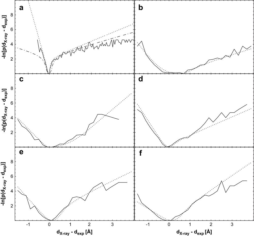
Negative logarithm of the normalized distribution of rref−rexp (solid line), a manually fitted symmetric function, (dashed line, only in (a)), and optimal fit (dotted line); (a) BPTI trajectory data, (b) Il4 [34,35], (c) BPTI [36,37], (d) pH domain [38,39], (e) GB1 domain [40,41], (f) Ubiquitin [42,43]. The dotted line represents a fit of the functional form (the “soft-square” potential) already implemented in X-plor [44] and CNS [45] to the negative logarithm of the distribution. Note the general similarity of the potentials, despite the differences in the used data sets with respect to completeness and quality. From Ref. [31], with permission.

RMS and RMSD values plotted against the level of added random noise added to the experimental distances for Ubiquitin, calculated with the potential from Fig. 4(a), and a data weight of 32. The values indicate the interval from which the random number was drawn; 0.2 indicates the interval [−0.2, 0.2] and so forth. Top panel: RMSwork (solid line) and RMScv (dotted line). Bottom panel: RMSDX-ray (solid line) and RMSDave (dotted line). Note that all the calculations were performed with exactly the same conditions, that is, in marked difference to other studies [16,24], values for the expected error did not have to be known before the calculation. From Ref. [31], with permission.
4.3 The lognormal distribution and a derived potential
Despite the robustness of the results to the exact shape of the potential, it may seem problematic to use a potential with several free parameters in addition to the overall weight. We discuss therefore another approach to the derivation, an error distribution and a restraint potential, from more fundamental properties of NOEs and derived distances. To this end, we analyse the expected deviation of a measurement from the ideal value. Although the original analysis [46] was performed for NOE intensities I, it is valid also for distances.
NOE intensities and derived distances are inherently positive. A calibration factor γ need to be introduced in order to relate the intensity scale to a distance scale. Changing the units does not affect the information content of the data. Hence, the distribution g(Iobs, Icalc) of the deviations between observed and calculated intensities must be invariant under scaling, i.e., g(Iobs, Icalc) = αg(αIobs, αIcalc), which follows from the transformation rule of probability densities. A distribution that shows this scale invariance is the lognormal distribution:
| (14) |
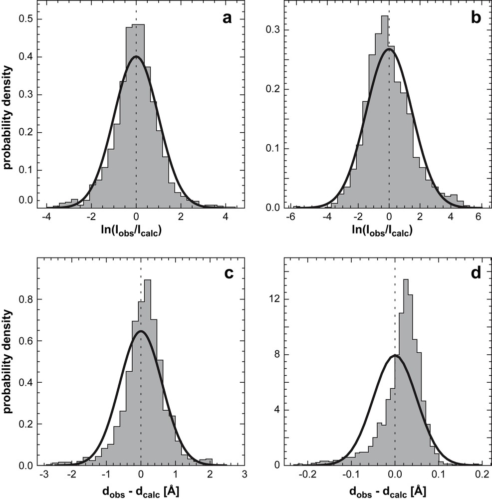
Experimental intensity error distributions for (a) Ubiquitin and (b) the Tudor domain. Solid lines indicate fitted lognormal distributions; (c) and (d) corresponding distance error distributions and fitted Gaussians. Because intensities were unavailable for Ubiquitin, we used the ISPA to convert the published distance data into intensities (1444 non-redundant distances taken from the restraint file, PDB code 1d3z). The Tudor data (1875 intensities from two 13C and 15N edited spectra) were calibrated such that observed and calculated values have the same geometric mean. From Ref. [46], with permission.
Fig. 6(c) and (d) shows distributions for distance differences dobs−dcalc fitted to a Gaussian distribution. The distance error distributions are asymmetric and long-tailed and a Gaussian can significantly underestimate the probability of large deviations. Both properties are much better accounted for by the lognormal distribution. From a practical point of view, the lognormal model has several favorable properties. Unlike a probability distribution corresponding to a flat-bottom potential, it has a unique maximum. Hence, measurements are not weighted equally between bounds but are always penalized depending on the degree of disagreement with the structure. Furthermore, the lognormal distribution is invariant under power law transformations. If we raise the intensity to a power the transformed intensity still follows a lognormal law, with transformed median and error parameters. Since the ISPA is a special case of a power transformation, we obtain identical distributions for intensities and distances, provided that σ has been transformed appropriately. The lognormal model is implemented in our software for probabilistic structure determination (ISD) for calculating the likelihood based on NOE intensities or NOE-derived distances.
The negative logarithm of the distribution in Eq. (14) is the corresponding restraint potential:
| (15) |
5 Data quality and the weight on Edata(X)
As already mentioned in Section 1, the weight plays a fundamental role in calculating structures from experimental data. Within ISD, the weight is estimated along with all the other unknown parameters (see above). In a standard structure calculation by minimisation, the experimental data are weighted empirically: wdata is set ad hoc and held constant during structure calculation. In their original paper, Jack and Levitt [1] proposed to adjust the weight so as to equalise Ephys and wdataEdata(X); this has been later refined to equalise average gradients [47]. In NMR, one usually uses fixed empirical values. In particular for the single minimum potentials discussed in the previous section, the weight has a profound influence on the results.
5.1 Setting the weight by empirical means: cross-validation
An unbiased empirical method to determine the optimal weight is cross-validation [48,49]. Data are divided into a working set, used to calculate the structure, and a test set, used only to evaluate the structure. Two measures of quality can be obtained: the RMS difference to the working set defines the usual fit to the distance restraints (or distance bounds), and the RMS difference to the test set defines a cross-validated measure that is not directly influenced by the data. If we measure the deviations from the distance (not from the bounds):
| (16) |
| (17) |
To determine optimal conditions for a structure calculation, we need to vary these conditions (in our case, the weight on the distance restraint term) and repeat structure calculations with otherwise unchanged conditions (around 100 structures for each weight, i.e., ten per test set). Often, RMScv does not show a clear minimum but an elbow, and it is convenient to define an optimal weight using the elbow region (e.g., as the point where there was less than 10% change in RMScv).
Fig. 7 shows, for Ubiquitin, the RMS differences and the WhatCheck [50] quality indices NQACHK and RAMCHK, as a function of the data weight used in the calculation. Around the optimal weight, calculations are not very sensitive to the precise value, and the elbow region is usually around values between 16 and 32, coinciding with the optimal values for RMS differences from the X-ray crystal structure, and for RAMCHK.

RMS differences and quality indices for Ubiquitin for calculations with the PDFMDman potential. Top panel: RMS difference from data RMSwork (solid line), cross-validated RMS difference from data RMScv (dotted line). Middle panel: NQACHK (solid line) and RAMCHK (dotted line). Bottom panel: RMS distance from the X-ray crystal structure RMSDX-ray (solid line) and RMS distance from average structure RMSDave (dotted line). Structures were calculated with the distance restraint potential shown in Fig. 4(a). From Ref. [31], with permission.
While cross-validation is an unbiased approach to obtain optimal parameters for a structure calculation, it is a rather insensitive to the parameter values. If many weights for different data terms need to be determined, its use becomes cumbersome, since many combinations of weights need to be evaluated. Another disadvantage is the necessity to remove data from the calculation, which, in the case of very sparse data, may reduce convergence.
5.2 Probabilistic approaches to set the weight
Probability theory gives us other possibilities to weight experimental data in an objective way: (i) the unknown weight parameter can be sampled along with the other unknown parameters, as in the ISD approach [26] described above; (ii) the weight can be included into the restraint function [51]; or (iii) the weight can be eliminated by marginalisation.
We focus on the second method, inclusion of the weight into a restraint function, since it is of most practical importance for minimisation. The negative logarithm of Eq. (11), the full posterior probability including the nuisance parameter σ is
| (18) |
The term log[Z(σ)/π(σ)] in the joint hybrid energy, Eq. (18), is not included in the standard target function Ehybrid, Eq. (1). However, it is precisely this additional term which allows us to determine the error. Z(σ) originates in the normalisation of P(D|X, I), π(σ) is required by Bayes's theorem. Both terms are missing in purely optimisation-based approaches, where normalisation constants and prior probabilities are usually not incorporated; this shows that a probabilistic framework is necessary for the correct treatment of the problem.
One might think that including the weight directly into a restraint energy would favour large values for σ with the corresponding weight approaching zero, since this would automatically minimise the restraint energy. However, the Bayesian analysis shows [51] that in the joint target function Ejoint, Eq. (18), two contributions counterbalance each other: χ2/σ2 decreases when σ increases, thus preferring large values for the error when Ehybrid is minimized with respect to the error. In contrast, the term log[Z(σ)/π(σ)] is monotonically increasing with σ (for the lognormal distribution, Eq. (14), it is ∝σn+1, where n is the number of data points). The ratio of the two terms therefore shows a finite minimum, which can be used to calculate the error, and, correspondingly, the optimal weight.
Minimisation of the resulting joint hybrid energy Ejoint(X, σ) yields the most probable structure Xmax and the most probable error σmax. In case of the lognormal model, Eq. (14), we obtain . Further analysis yields for the average weight as an estimate. These estimates concur with common sense: the average weight quantifies, in good approximation, how well the structure fits the data, independent of the size of the data set. The precision of the estimate, i.e., the width of the weight distribution, in contrast, decreases with the square root of the number of data points [51]. Therefore, when sampling the weight, we obtain sharp distributions for σ for typical NMR data (see Fig. 2). This estimate is much more precise than what we can obtain from cross-validation.
To apply this estimate in the context of structure determination by minimisation, we can iteratively update the current weight to . This weight is a conservative estimate since it is always smaller than χ2(Xmax)/(n + 1), the most probable weight derived from the most probable structure. We are at present testing implementations of this simple rule within CNS and ARIA.
6 Conclusions
In this paper, we reviewed approaches to obtain molecular coordinates from experimental data, with a special emphasis on treating it as a data-analysis problem of parameter fitting. Only the inferential structure determination method ISD satisfies the three conditions for a good fitting procedure mentioned in Section 1 in that it provides fitted parameters, error estimates of the parameters, and a statistical measure of a goodness of fit. It is the only method that can derive these estimates for the coordinates taking into account uncertainties in all additional parameters that are necessary for the structural modelling. It does not require prior estimates of data quality, but only information on the general form of the error distribution of the data. It can therefore be regarded as the “king's way” to structure calculation.
Least-squares type methods have the disadvantages that one must define experimental errors a priori, and that they impose a uni-modal Gaussian distribution on the resulting structures. In contrast, the standard way of estimating structural uncertainty by repeated structure calculations does not impose any distribution on the structures but suffers from the problem that the structural ensembles are largely influenced by algorithmic properties.
Despite the success of ISD, standard structure determination by minimisation will undoubtedly continue to play a dominant role in practical applications. We argue that, to obtain the maximum benefit, these approaches should derive from a rigorous probabilistic treatment. This has implications on the restraint potential and on the weighting of experimental evidence. For example, the necessity of defining the data quality a priori can be removed. Whereas we cannot get statistically meaningful coordinate uncertainties from the minimisation approach, our experience shows that the uncertainties in the structure determination automatically depend on the data quality if an appropriate restraint potential is used. We also foresee that the analysis of differences between experimental and calculated data on a per-restraint or per-residue basis will be more informative than with the presently used fixed weights and FBHW potentials.