

1 Introduction
A record 38% ozone depletion of about 160 DU, comparable in magnitude to that of the Antarctic, occurred in the Arctic winter 2011 (Adams et al., 2012; Arnone et al., 2012; Griffin et al., 2018; Lindenmaier et al., 2012; Manney et al., 2011; Pommereau et al., 2013; Sinnhuber et al., 2011). It was attributed to an unusually persistent polar vortex that lasted until the end of March. More recently, a 27% (120 DU) depletion, the third largest in magnitude since the beginning of SAOZ (“Système d’Analyse par Observation Zénithale”, Pommereau and Goutail, 1988) ozone column observations in 1990, occurred in the winter 2015–2016. In that year, the strongest and coldest polar vortex of the last 68 years was observed during a period of reduced @planetary wave (PW) amplitude (Matthias et al., 2016; Rex et al., 2016). As shown by the Aura Microwave Limb Sounder (MLS), such record low temperatures resulted in exceptional vortex-wide dehydration between the 410 K and 520 K potential temperature levels, somethingnever observed before in the Arctic. The observed denitrification was also exceptional, and extensive chlorine activation and chemical ozone loss began earlier than in the recent high loss winters. However, the magnitude of chemical ozone depletion was limited by an early major final warming at the start of March (Manney and Lawrence, 2016).
The question is therefore to understand whether the frequency of the anomalously cold and strong vortex conditions will increase in the future and thus persistently create conditions for large chemical ozone loss. The future frequency of these episodes will be influenced by the continuous cooling of the stratosphere through increasing concentrations of greenhouse gases (GHGs), as predicted in chemistry–climate models (CCMs). These processes can delay the Arctic ozone recovery currently predicted by CCMs for the mid-2030s (Dhomse et al., 2018; WMO, 2014). Using the ECHAM/MESSy Atmospheric Chemistry (EMAC) CCM, Langematz et al. (2014) suggested that the future Arctic stratosphere would cool significantly in early winter. Using the Met Office Unified Model–United Kingdom Chemistry and Aerosol (UMUKCA) CCM, Bednarz et al. (2016) confirmed to some extent the predicted cooling of the middle and upper stratosphere, but also underlined the low confidence in the projected temperature trends in the lower stratosphere. In addition, like Langematz et al. (2014), they confirmed the possible occurrence of significant episodic large ozone column reductions because of the large interannual dynamical variability of the Arctic atmosphere.
The objective of this paper is to investigate whether there are indications that Arctic ozone recovery, currently predicted for 2030–2040 (Dhomse et al., 2018; WMO, 2014), might be delayed and whether large episodic depletions might still occur following the cooling of the lower stratosphere predicted by the climate models. Section 2 provides an update of recent ozone loss and denoxification events observed by the SAOZ network in 2015–2016 and 2016–2017. The temperatures recorded in the Arctic vortex during these years are described in Section 3. The possible impact of the further predicted cooling of the stratosphere on ozone is then discussed in Section 4, and our conclusions are summarized in Section 5.
2 Ozone loss in 2015–2016 and 2016–2017
The ozone loss is derived from SAOZ column observations at eight stations in the Arctic (Table 1), where measurements are performed twice daily at solar zenith angles (SZAs) between 86 and 91°. Thus our observations extend up to the polar circle at the winter solstice. Table 1 shows the latitude and year of the first observations at each station.
SAOZ Arctic stations, latitude, longitude and year of first observations.
| Eureka, Nunavut | 80° N, 86° W | 2006 |
| Ny-Alesund, Svalbard | 78° N, 12° E | 1991 |
| Thule, Greenland | 76° N, 69° W | 1991 |
| Scoresbysund, Greenland | 71° N, 22° W | 1991 |
| Sodankyla, Finland | 67° N, 27° E | 1990 |
| Salekhard, Russia | 67° N, 67° E | 1998 |
| Zhigansk, Russia | 67° N, 123° E | 1992 |
| Harestua, Norway | 60° N, 11° E | 1994 |
The ozone loss and the amplitude of the NO2 diurnal variation reported during the winters of 2015–2016 and 2016–2017 are shown in Fig. 1. The ozone loss at each station is calculated by a passive method where measured columns are compared to those provided by chemical transport models (CTMs) that ignore chemistry, as described by Goutail et al. (1999). Griffin et al. (2018) recently showed that this method provides smaller uncertainties in ozone loss calculations than other approaches. Also displayed in Fig. 1 is the nitrogen dioxide (NO2) diurnal variation, an indicator of chlorine activation. Indeed, since NOx is transformed into ClONO2 in the presence of activated chlorine, the absence of NO2 during night time is an indicator of chlorine activation (Pommereau et al., 2013). During the winter 2015–2016, the afternoon NO2 levels remained low until the end of February, when the chlorine activation stopped and the ozone column depletion reached a total of 27 ± 3% on March 20, at a mean rate of 0.5%/day. In contrast in the winter 2016–2017, the chlorine-activated period was shorter and ended in late January, the loss rate was smaller at 0.2%/day, and the total ozone depletion amplitude reached only 16 ± 3%.
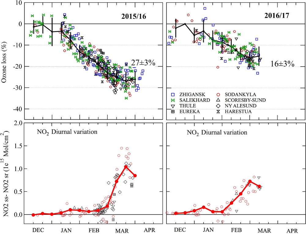
Time series of observed ozone loss (%) inside the vortex (top panels) and the amplitude of the NO2 diurnal variation (bottom panels), above each SAOZ station in winter 2015–2016 (left) and in winter 2016–2017 (right).
The long-term history of the ozone loss since the beginning of SAOZ network measurements in 1990 and the results of the CTMs REPROBUS (Lefevre et al., 1994) and SLIMCAT (Chipperfield, 1999) are shown in Fig. 2. Although stopped by the major stratospheric final warming in early March, the 2015–2016 ozone depletion is the third largest after the peak of 1995–1996 and the record loss of 2010–2011. Remarkably, cases of small ozone depletion, which were frequent between 1998 and 2005 due to early warmings in late December or early January, are no longer observed after 2005. As shown by the EMAC model simulations, this is consistent with the early winter cooling of the stratosphere below the threshold temperature of nitric acid trihydrate (NAT) PSC formation (TNAT) observed every winter after 2005, resulting in a minimum ozone depletion of at least 12–15% each year.
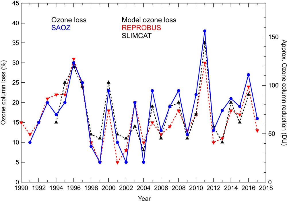
Ozone column loss magnitude (%) reported by the SAOZ network each year since 1990 and calculated by the two chemical transport models REPROBUS and SLIMCAT.
Regarding the CTM simulations with interactive chemistry, the depletion amplitudes of 27 ± 3% in 2015–2016 and 16 ± 3% in 2016–2017 are well captured by the models with, respectively, 24.3 ± 1.9% and 13 ± 2% in REPROBUS, and 25 ± 2% and 11 ± 2% in SLIMCAT. An exception to the good agreement over the recent SAOZ record is in 2012–2013, when both models significantly underestimate the observed ozone loss.
Fig. 3 shows the relationship between SAOZ ozone loss amplitude and NAT polar PSC illuminated (sunlit) volume. The NAT PSC sunlit volume is calculated in the lower stratosphere between 400 and 675 K potential temperature surfaces (Pommereau et al., 2013). The 2015–2016 and 2016–2017 episodes are fully consistent with the other winters, confirming the linear relationship between ozone loss and NAT PSC sunlit volume, indicative of chlorine activation (Chipperfield et al., 2005; Pommereau et al., 2013; Rex et al., 2004).
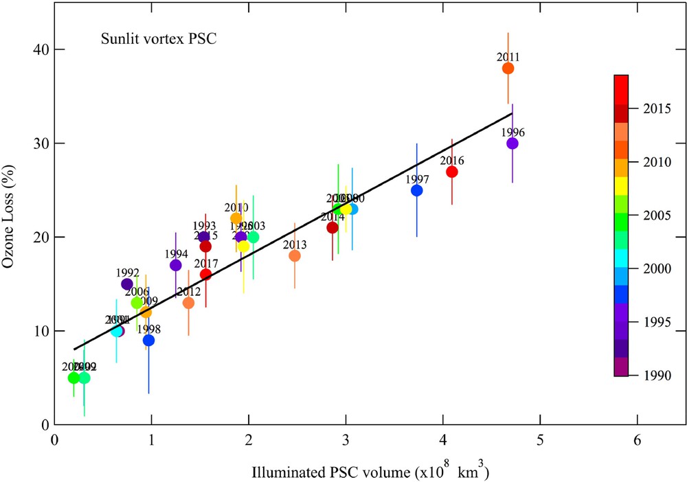
Magnitude of SAOZ ozone loss (%) versus nitric acid trihydrate (NAT) PSC sunlit volume (VPSC) between the 400–675 K levels.
3 Stratospheric temperatures in the winter Arctic
Fig. 4 shows the minimum ECMWF ERA-Interim temperatures at the 475 K isentropic level (approximately 18 km), reported each winter since 1990 north of 60° N. The bold blue line is for winter 1996, when the second largest ozone loss so far observed occurred. The bold black line is for the record loss of 2010–2011, the red line for 2015–2016, and the green line for the relatively warm 2016–2017 winter. Also shown are TNAT and the ice PSC formation temperature (TICE).
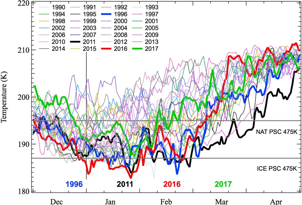
ERA-Interim minimum temperature north of 60° N at the 475 K level between December and April for winters from 1989–1990 to 2016–2017.
As already noted, the early stratospheric warming in December and January observed frequently before 2005 did not occur after 2005, which is consistent with the model study of Langematz et al. (2014). The temperature is often below TNAT for several weeks. However, apart from short-duration ice PSC episodes associated with mountain-wave events, like those observed by the ALOMAR lidar in northern Norway in January 1996 (e.g., Hansen and Hoppe, 1997), a long duration period with T < TICE happened recently only (Fig. 4). The first significant T < TICE episode, which lasted two weeks after mid-February in the winter 2010–2011, resulted in the record ozone loss event. A T < TICE event like the most recent, which lasted for one month in January 2016, had never been observed before in the Arctic. This January 2016 event resulted in the fast sedimentation of ice particles leading to the unprecedented dehydration and denitrification of the stratosphere (Manney and Lawrence, 2016) and the complete denoxification until late February, as observed by SAOZ (Fig. 1).
4 Discussion
The winters 1995–1996, 2010–2011, and 2015–2016 have been the coldest so far since the beginning of SAOZ observations, and they resulted in the largest observed ozone losses. Although Arctic stratospheric ozone recovery is predicted to occur in the mid 2030s, there is no indication yet of reduced ozone loss at northern polar latitudes, in contrast to the Antarctic (Solomon et al., 2016). Arctic ozone depletion typically amounts to 12–15% (30–50 DU) each year, reaching 25% (60 DU) during moderately cold winters, can be as large as 38% (160 DU) in extreme cases. Since there is a clear relationship between stratospheric temperature and ozone loss while stratospheric chlorine and bromine loadings remain elevated, if the cooling of the stratosphere continues, there is a serious risk of experiencing further extreme loss events before the concentrations of ozone-depleting substances (ODSs) return to their pre-depletion values. The question is thus to understand how the temperature of the Arctic lower stratosphere will evolve in the future.
Using Chemistry–Climate Model Initiative (CCMI) EMAC simulations, Langematz et al. (2014) concluded that the lower stratosphere minimum temperature (Tmin) north of 40° N is decreasing in the early winter (November–December) at a mean rate of −0.18 ± 0.05 K/decade since 1960, but at a slightly slower rate (−0.11 ± 0.05 K/decade) in January–February. According to their predictions, the cooling will continue until 2100. Using ECMWF ERA-Interim and NASA MERRA meteorological reanalysis datasets, Bohlinger et al. (2014) also studied long-term stratospheric temperature changes. They found that the Arctic lower stratosphere at 50 hPa between 60–90° N has been cooling, faster than predicted by the EMAC model, at a rate of −0.41 ± 0.11 K/decade over the last 32 years. Like Langematz et al., Bohlinger et al. also suggested a further cooling of the Arctic stratosphere over the coming decades due to radiative cooling largely controlled by the changes in GHGs, but at slower rate of −0.15 ± 0.06 K/decade for EMAC and −0.10 ± 0.02 K/decade for the Climate Validation (CCMVal2) project. Finally, from the seven-member ensemble simulations of the UMUKCA, Bednarz et al. (2016) also concluded that there would be a statistically significant long-term cooling throughout most of the polar stratosphere in early winter, in agreement with Langematz et al. (2014). The results also indicate a strengthening of the deep branch of the Brewer–Dobson circulation in boreal winter (Hardiman et al., 2014), implying an increase in downwelling over the Arctic from December to February of 0.015 ± 0.007 mm/s/decade. Regarding ozone, the ensemble model simulations lead to the conclusion that although the total column in March is expected to increase at a rate of 11.5 DU/decade in the 21st century, the springtime Arctic ozone can episodically drop by 50–100 DU, meaning that individual years with springtime ozone depletion as severe as that of 2011 will remain possible in the future. Furthermore, Sun et al. (2014), using the Whole Atmosphere Community Climate Model (WACCM), have shown that the predicted sea ice loss in the Arctic could lead to a decrease of the upward wave propagation, a strengthening of the polar vortex, an additional cooling of the stratosphere, and then a polar cap stratospheric ozone decrease by 13 DU (34 DU at the North Pole) in spring. Using CCMI results, Morgenstern et al. (2017) examined the degree of consistency in column ozone predictions between seven models and found considerable disagreement, which they attribute to inter-model differences in lower stratospheric transport and dynamical responses. They concluded that there is a lot of uncertainty in the future evolution of temperature. Finally, from the more recent 155 simulations performed by 20 models in the in the frame of CCMI, Dhomse et al. (2018) concluded that the return dates of ozone to the 1980 level, will be later by approximately 5–17 years than those presented in the 2014 Ozone Assessment. However, like Morgenstern et al., they also found a significant uncertainty in the predictions.
5 Conclusions
In conclusion, all model predictions agree with a further cooling of the Arctic lower stratosphere due to increasing GHG concentrations. However, significant differences in the model skill are found, e.g., prediction of the cooling episodes limited to the early winter or extending through the whole winter, cooling limited to the middle and upper stratosphere or extending to all levels, related to the strengthening or weakening of the Brewer–Dobson circulation, or additional stratospheric cooling after sea ice melting, etc. Generally speaking, model predictions are consistent with the observed cooling of the lower stratosphere during the winter, consistent, for example, with the recent low temperature record of 2015–2016. CCMI simulations also agree with the relationship between temperature and ozone loss, for which observations are well captured by chemical transport models. The high variability of Arctic meteorology implies that large chemical ozone depletion events like those of 2010–2011 and 2015–2016 might still occur until the ODS concentrations return to their 1960 values. The Arctic stratospheric ozone recovery predicted for the mid 2030s might be thus significantly delayed.
Most important in order to predict the future Arctic ozone evolution and reduce the uncertainty of the timing for ozone recovery is to ensure continuation of high-quality ozone observations in the Arctic with adequate instruments, UV-Vis ground-based (Pommereau et al., 2013), radiosondes (Rex et al., 2004), Microwave MLS (Waters et al., 2006) and IR IASI (Boynard et al., 2018), performing at high latitude in winter.
Acknowledgments
The authors are indebted to the personnel operating the SAOZ/NDACC stations and Cathy Boone at the French AERIS/ESPRI data centre http://www.cds-espri.ipsl.upmc.fr/ for providing MIMOSA, REPROBUS and ECMWF analyses and reanalyses. The SAOZ measurements at Eureka/CANDAC are supported by the Canadian Space Agency. The SAOZ data are available at the NDACC data centre http://www.ndsc.ncep.noaa.gov/. This research is supported by the NDACC French programme funded by the “Institut national des sciences de l’Univers” (CNRS/INSU), the “Centre national d’études spatiales” (CNES) and the polar Institute Paul-Émile-Victor (IPEV), which are gratefully acknowledged. The SLIMCAT modelling work is supported by the National Centre for Atmospheric Science (NCAS).