


 CC-BY 4.0
1. Introduction
With a local magnitude (ML) of 5.4 (CEA-DASE, Commissariat à l’Energie Atomique et aux Energies Alternatives—Département analyse, surveillance, environnement) and a moment magnitude (Mw) of 4.9 [Cornou et al. 2021; Ritz et al. 2020], the 11 November 2019 Le Teil earthquake (10h52 UTC) is one of the strongest and most destructive earthquakes that occurred in the last decades in metropolitan France.
The source of the Le Teil earthquake has been the object of several studies [Delouis et al. 2019; Cornou et al. 2021; Ritz et al. 2020; De Novellis et al. 2020; Mordret et al. 2020], from which a detailed picture of the coseismic rupture emerges. The rupture was ∼5 km long, trending NE–SW, reaching the surface, with reverse fault motion uplifting the SE side of the fault, as first evidenced by a synthetic aperture radar interferogram (InSAR) in agreement with the focal mechanism obtained from the first waveform inversions. Surface breaks were observed in the field along ∼5 km, consistent with reverse faulting, with up to 15 cm of uplift of the SE side of the fault. The rupture was shallow, with slip located essentially between the surface and 1 km depth, as constrained by the InSAR data and waveform inversions. The La Rouvière fault, trending NE–SW and dipping to the SE, was identified as the causative fault of the earthquake. A bilateral rupture was inferred from the analysis of seismological data.
Despite the overall characteristics depicted by those studies, the location of the mainshock hypocenter remains poorly determined, because the earthquake occurred in a region of scarce seismicity and sparsely instrumented by permanent seismological stations. As reported by Delouis et al. [2019] and Cornou et al. [2021], the mainshock epicenters determined based on the permanent velocimetric network were systematically located NW of the La Rouvière fault trace. Since the fault is dipping to the SE, those epicenter estimates were spuriously shifted to the wrong side of the fault by up to several kilometers (Figure 1). Another reviewed location proposed by the LDG and based on a large number of regional stations also places the epicenter on the wrong side of the fault [Vallage et al. 2021]. A relocation of the mainshock hypocenter is hence required in order to determine where on the La Rouvière fault the rupture initiated, and to compare the result with analyses based on independent observations which pointed to a bilateral rupture [De Novellis et al. 2020; Causse et al. 2021; Mordret et al. 2020].
The shallow hypocenter and its proximity to a large limestone (cement) quarry raised the question of the possible relationship between the extraction of rocks and the triggering of the earthquake. This point was first addressed by Delouis et al. [2019], then by Liang and Ampuero [2020] and De Novellis et al. [2020, author correction, 2021]. Analyzing in more detail this relationship is not in the scope of the present paper, but the relocation of the mainshock initiation area is one of the elements to be considered in this matter.
Map showing the early routine epicenters of the Mw 4.9 mainshock (red stars) determined by various agencies (indicated by their acronyms), redrawn from Cornou et al. [2021]. The green star is the epicenter of the 23 November 2019 aftershock (Ml 2.8) located with the dense post-seismic network (this study), and used as a master event. Heavy black line with triangles: simplified trace of surface breaks, triangles pointing in the dip direction (SE) of the reverse fault that ruptured during the Le Teil earthquake. Gray shaded area: approximate contour of the limestone (cement) quarry. Background map from the French Geoportal, IGN, https://www.geoportail.gouv.fr/carte.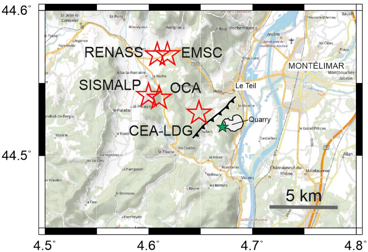
A preliminary attempt to relocate the mainshock hypocenter was carried out by Delouis et al. [2019] by incorporating additional stations in the epicentral region, either belonging to temporary experiments initiated before the Le Teil earthquake [e.g., AlpArray, Hetényi et al. 2018] or whose data were not transmitted in real time to the national or international data centers the day of the earthquake. These stations were made available in the days following the earthquake by the AlpArray project, the Institut de Radioprotection et de Sûreté Nucléaire (IRSN), and (Électricité de France (EDF).
Despite the usefulness of such additional stations, which provided some recordings closer to the rupture (8 to 20 km instead of >30 km for the permanent network), it was possible to locate epicenters on the correct side of the fault only by restraining hypocentral depth in the range 1 to 1.5 km, by using a high value of the Vp∕Vs ratio, between 1.8 and 1.9, and by using only the four closest stations. The depth range 1 to 1.5 km was imposed according to the results of preliminary InSAR and waveform inversions. The epicentral solutions obtained in this first study are not completely satisfactory since they resulted from very specific constraints imposed in the inversion of seismic wave travel times.
In the present study, we aim at determining the epicentral location and the depth of the Le Teil mainshock exclusively from the P and S arrival times, without a priori constraint on the depth range. In the absence of nearby stations having recorded the mainshock at distances shorter than 8 km, we use specific strategies such as the master event technique or other relative location techniques. We also give a specific attention to the optimization of the velocity model.
Routine determinations of hypocenters in France rely on one-dimensional (1D) velocity models which have been defined at the national or at a broad regional scale [CEA-DASE, Duverger et al. 2021; BCSF-RENASS, Bureau Central de Sismologique Français — Réseau National de Surveillance Sismique, Cara et al. 2015]. Although they have been validated as well-performing average models, they cannot reflect local variations in seismic wave velocities that may take place in areas of contrasted geology. Three-dimensional (3D) velocity models have been determined for some regions in France [e.g., [Potin 2016] for the Alps and [Bethoux et al. 2016] for the southern Alps and Ligurian basin]. A preliminary 3D velocity model has been produced at the scale of metropolitan France [Arroucau 2020], but its real potential for improving the quality of the hypocentral solution has yet to be evaluated. In many regions of France, and in particular, in the region of the Le Teil earthquake, the velocity structure may still have a large uncertainty, especially at the scale of a few tens of kilometers.
We developed a specific hypocentral location approach to take into consideration such level of uncertainty, combining a nonlinear exploration of the hypocenter parameters with an exploration of the velocity model.
We called the method GRIDSIMODLOC as it combines a grid search, a simulated annealing, and an optimization of the 1D velocity model. In recent years, this method, combined with the FMNEAR waveform inversion also used in the present study [Delouis 2014], has been applied to several earthquakes of moment magnitude Mw 3.2 to 4.9 in France and results have been published on the BCSF special events web pages [e.g., BCSF 2018, 2019a,b, 2020]. The GRIDSIMODLOC method is first described in this paper and applied to the Le Teil mainshock and its 23 November 2019 aftershock.
Our first tests show that whatever the 1D velocity model used, hypocenter solutions obtained by inverting P and S arrival times, without the specific constraints imposed by Delouis et al. [2019], tend to be located on the NW side of the fault. Using a set of stations evenly distributed around the epicenter does not solve this issue, suggesting that the bias in location cannot be explained by the configuration of the seismic network. Alternatively, a systematic bias in location can be explained by a lateral contrast in seismic wave velocity unaccounted for when using a 1D velocity model by which hypocenters are shifted toward the area of higher velocity. A simple illustration and explanation of this situation can be found in Havskov et al. [2012].
In our search for an unbiased mainshock location, we followed two different strategies: (1) use of the master event technique, and (2) search for a dual velocity model, geographically split in two subregions. As a master event, we will mainly rely on the 23 November 2019 (22h14 UTC) aftershock of local magnitude ML 2.8 (SISMALP, Réseau d’observation de la sismicité Alpine) but we will also make use of a quarry blast in the vicinity of the mainshock. The aftershock has been particularly well-recorded by the temporary post-seismic network, and it is one of the largest aftershocks of the Le Teil seismic sequence.
Focal mechanisms determined by waveform inversion for the Le Teil mainshock in the days following its occurrence, as summarized on the European-Mediterranean Seismological Centre (EMSC) web page (https://www.emsc-csem.org/Earthquake/earthquake.php?id=804595#map) concur in the dominant reverse faulting component, with NE–SW nodal planes. However, they display large variations in the dip angles (37° to 57°) and in the depth (1 to 13 km). In this study, we revisit the focal mechanism of the Le Teil mainshock by waveform inversion, in terms of double-couple solution and deviatoric solution of the moment tensor, with two different approaches and different velocity models, so as to investigate in detail the dip and depth parameters. The analysis is complemented by the determination of the focal mechanism of the mainshock and its aftershock with the available first motion data.
2. The GRIDSIMODLOC method
The hypocenter parameters (latitude, longitude, depth, and origin time) are explored with a nonlinear travel time inversion combining a grid search, a simulated annealing algorithm, and the Hypoinverse-2000 program [Klein 2014].
First of all, bounding values are prescribed for latitude, longitude and depth. Those are generally based on an initial hypocentral location and an estimation of the associated uncertainty. This defines the search area for the grid search and simulated annealing explorations. If necessary, the search area can be adjusted after an initial inversion, especially if the best solutions are found to lie close to the boundaries of the search area.
Exploration involves three interlocked loops. The first outer loop scans different crustal velocity models. The second intermediate loop explores the three location parameters latitude, longitude, and depth one by one, setting the current explored parameter to successive values between its lower and upper limits with a prescribed increment. We call this step the 1D grid search. In the third innermost loop, the parameter explored in the 1D grid search is maintained fixed and the other two location parameters are optimized with a simulated annealing algorithm. At the heart of this third and last loop, the Hypoinverse-2000 program [Klein 2014] is called to calculate the theoretical travel times, adjust the earthquake origin time, and provide the time residuals with the corresponding root mean square (RMS) travel time misfit function. The RMS value constitutes the cost function that must be minimized.
The aim of the 1D grid search is to map the hypocenter solutions with their respective RMS values all along the prescribed intervals of the searched parameters. The overall nonlinear inversion combining 1D grid search and simulated annealing obviously requires more computing than the linearized inversion implemented in Hypoinverse-2000 [Klein 2014], but it provides an extensive mapping of the parameter space allowing a better uncertainty assessment. It is also essentially independent from any initial solution.
For the Le Teil earthquakes, bounding intervals for latitude, longitude, and depth are [44.49, 44.56°], [4.6, 4.7°], [0.2, 15 km], respectively. The increments in the 1D grid search are 0.002°, 0.002°, and 0.2 km in latitude, longitude, and depth, respectively.
The Earth structure is represented by a single crustal layer with a constant linear velocity gradient, overlying a homogeneous mantle. Crustal thickness and mantle velocity are fixed. In the case of the Le Teil earthquakes, these two parameters are set to 30 km and 7.9 km/s, respectively. Moho depth was chosen as an average value for the area based on the Moho map from Ziegler and Dèzes [2006]. However, for the location purpose, mantle parameters will not matter in the end, since we will obtain our final location of the Le Teil earthquake with stations located at short epicentral distance (<50 km) for which first arrivals are only from direct wave paths. With this kind of models, station elevations are taken into account in the location process [Hypoinverse-2000 program, Klein 2014].
The choice of a 1D constant velocity gradient model rather than a 1D model made by multiple layers with homogeneous velocity is motivated by the determination of the focal mechanism with first motion data. With a constant gradient model, the incidence angle of the seismic ray at the source varies smoothly with epicentral distance. This generally results in the determination of a stable focal mechanism solution. On the contrary, multi-layered models can produce abrupt discontinuities in the incidence angle around specific epicentral distances for which the seismic ray flips from a direct path to a refracted path along one of the crustal layer discontinuities. As a result, a small change in the hypocentral depth, or a small change in the depth of a particular layer interface in the model, can strongly affect the incidence angles and lead to a different focal mechanism solution or a focal solution with more apparently incoherent P first motion observations.
Within the Hypoinverse-2000 program [Klein 2014], we define the 1D linear velocity crustal model by the P wave velocity at the top of the crust, the velocity gradient in km/s/km, a constant Vp∕Vs ratio, and crustal thickness. Instead of reporting velocity gradient values which are somewhat abstract, we will report the P wave velocities at the top and bottom of the crust, acknowledging that the velocity is indeed linearly increasing in between. After some preliminary trials, we allow the P wave velocity at the top of the crust to take the following discrete values 4.5, 5.0, and 5.5 km/s. At the bottom of the crust, the discrete explored values are 6.6, 6.8, and 7.0 km/s. The crustal Vp∕Vs ratio varies between 1.66 and 1.9 with a 0.03 increment, consistent with preliminary tests showing a tendency to favor high values of Vp∕Vs ratio. In the mantle, the Vp∕Vs ratio is fixed to 1.73. The number of velocity models tested when combining all these discrete values is 3 × 3 × 9 = 81.
It is a fact that crustal velocity models are poor representations of the actual crust, and therefore hypocentral locations can always be considered biased to some extent. There exist different ways to try reducing this bias. Widely used approaches include the search of an optimum (minimum) 1D velocity model combined with station corrections [e.g., VELEST, Kissling et al. 1994], seismic tomography to obtain a 3D velocity model suitable for earthquake location [e.g., Paul et al. 2001], probabilistic nonlinear location methods incorporating 3D velocity models [e.g., Lomax et al. 2000, 2009]. However, in many places around the world, including France, such refined models are not available, especially where earthquakes are rare and seismic stations sparse.
Here we choose to follow a different approach. Acknowledging that the crustal structure is poorly known, a wide range of physically plausible velocity models are tested. The drawback of such approach is that it tends to maximize the hypocentral location uncertainty with respect to what would be obtained with a velocity model precisely adapted for the area under consideration. On the other hand, if the resulting hypocentral solutions show a low degree of scattering, then these solutions can be considered as stable whatever the velocity model. Of course, the final solutions obtained with the optimized 1D velocity model may be biased if the true Earth structure below the stations exhibits a strong lateral velocity contrast, as we will infer to be the case in the region of the Le Teil earthquake.
Strategy followed using the aftershock located with the dense post-seismic network as the master event. On the top left map, the light gray area with a black contour shows the approximate area of the limestone (cement) quarry, and the black line is the simplified trace of the mainshock surface breaks.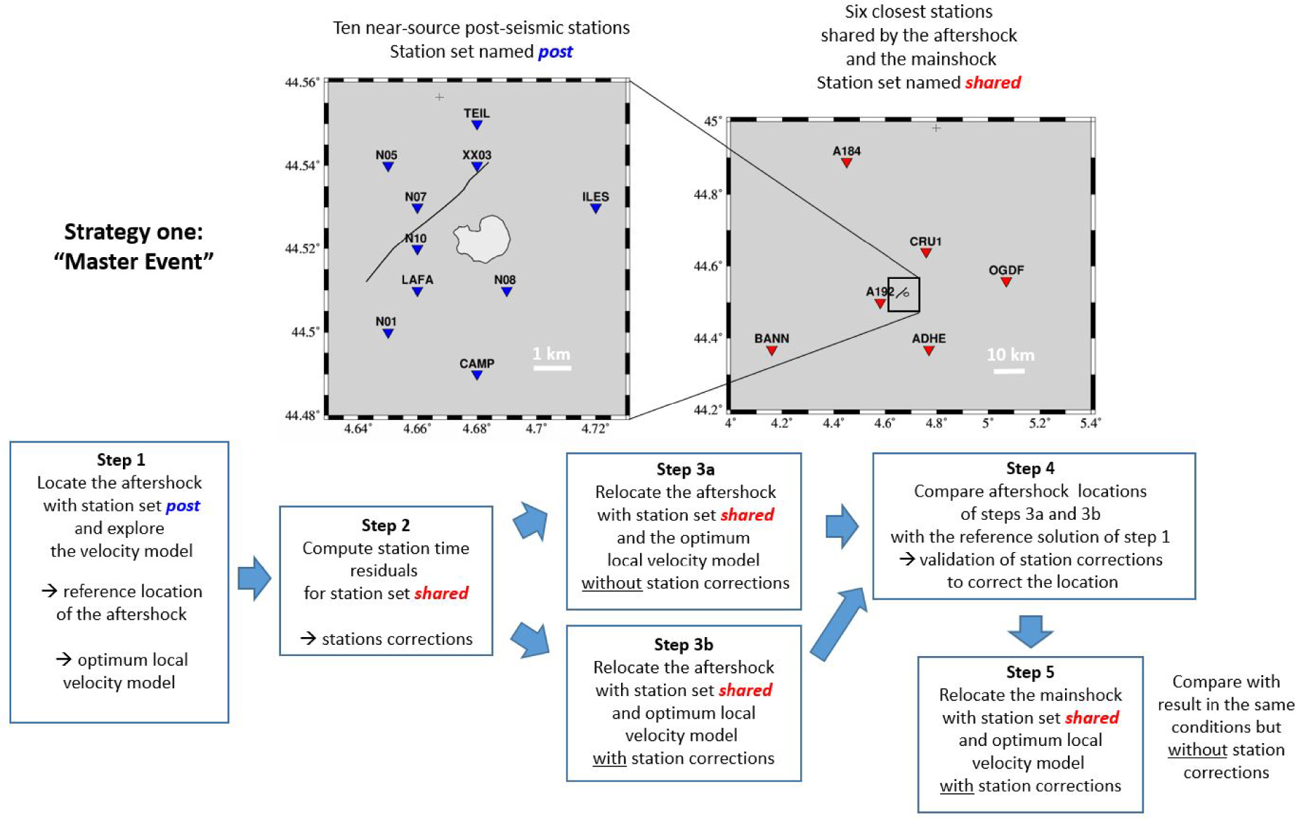
Result of the GRIDSIMODLOC inversion for the aftershock using the post-seismic network of ten stations (post), corresponding to step1 of Figure 2. (a) RMS of time residual as a function of latitude, longitude, and depth. The red dashed line shows the threshold (RMS = 0.05) used to represent the best solutions in (b) and (c). (b) Map view and (c) NW–SE cross-section perpendicular to the fault strike. Circles are the best solutions, filled in green when compatible with the fault dipping between 40 and 65° to the SE. On map (b), the light gray area with a black contour shows the approximate area of the limestone quarry, and the black line is the simplified trace of the mainshock surface breaks. Note: green solutions are displayed for the aftershock though it did not necessarily occur on the main fault (see discussion). The orange star is the average hypocenter. (d) 1D velocity model providing the lowest RMS values, called the optimum local velocity model in Figure 2 and in the text.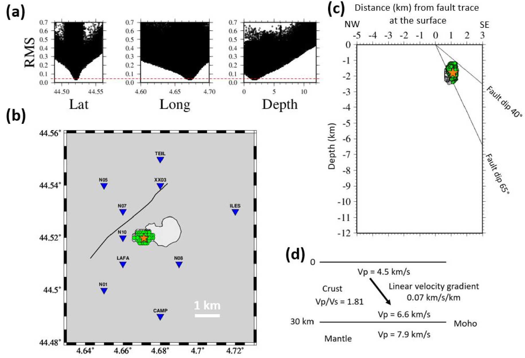
3. Relocation of the mainshock using the aftershock as a master event
The strategy followed to relocate the Le Teil mainshock using the aftershock as a master event is summarized in Figure 2. In the first step, we select two sets of stations. The first set is called “post” and comprises ten temporary post-seismic stations all within 5 km distance from the rupture area. Deployed during the first two weeks following the mainshock, they constitute an optimal network that recorded the aftershock but not the mainshock. The second set is called “shared” as it comprises six of the closest stations that recorded both the mainshock and its aftershock. These six stations minimize epicentral distances (between 8 and 45 km) and optimize the azimuthal coverage. Considering the much denser and closer network post, the location of the aftershock is much better constrained, and consequently, the ML 2.8 aftershock is taken as the master event. Most of the seismological data are available through the French RESIF (Réseau Sismologique et Géodésique Français) data portal (http://seismology.resif.fr/) or the European Integrated Data Archive (EIDA) portal (http://www.orfeus-eu.org/data/eida/). Additional seismic records were provided by EDF and IRSN (available through the RESIF data portal), as well as by the AlpArray temporary experiment [AlpArray 2015, restricted access].
We read the P and S arrival times at all stations of the “post” and “shared” sets for the aftershock, and “shared” set for the mainshock. To better assess the S wave onset times, we carry out analyses of the horizontal polarization (particle motion) in a window moving around the initially read S arrival time, and picked the time when a clear change in polarization direction occurred (see example in Figure S1, Supplementary Material). We adapt the weights of the phase data according to the impulsive or emergent character of the wave onset and change in horizontal polarization for the S wave. If the polarization change is sharp in time and unambiguous, a phase weight of 1 is assigned to the arrival S. This weight is changed to 2 if the polarization change is less sharp and to 3 if it is more ambiguous but still identifiable. Note that the actual weight of a given phase in the localization process is equal to (4—phase weight).
In a first step, the aftershock is located with station set “post” using the GRIDSIMODLOC approach (step 1 in Figure 2). The result is displayed in Figure 3. RMS values exhibit a peaked distribution as a function of the three hypocentral parameters, meaning that the hypocenter is effectively well constrained. The best solution found is at 44.5200 N, 4.6718 E, 1.7 km depth, and origin time 22:14:54.62 (HH:MM:SS.S), with an RMS value of 0.04 s. Considering solutions with RMS values smaller than 0.05, a group of solutions is obtained, closely spaced around an average hypocenter at 44.5198 N, 4.6713 E, and 1.8 km depth (Figure 3b and c). Note that the RMS threshold at 0.05 is not based on a strictly objective criterion, we simply consider that RMS values between 0.04 and 0.05 are almost indiscernible from the point of view of data fitting.
Solutions below the chosen RMS threshold can be considered as almost equiprobable since the variation of RMS among them is very small (typically <0.03 s). For that reason, we highlight the average solution instead of the solution with the lowest RMS value which may occupy an eccentric position within the cloud of the equivalent solutions.
We acknowledge that the uncertainties in hypocenter location considered throughout this study and which are related to RMS thresholds are affected by a certain degree of subjectivity. For this reason, we show the RMS distributions in Figures 3(a) and Supplementary Material S2.
Given the 37°–57° dip values for the SE-dipping nodal plane of the moment tensor solutions compiled on the EMSC website (see introduction), the focal mechanism determinations realized in this paper (following sections), and the preferred dip of 50°–60° to model the InSAR data [Delouis et al. 2019; Cornou et al. 2021; De Novellis et al. 2020], we chose the 40°–65° dip range to determine if the hypocentral solutions are compatible with the causal fault geometry. This range could have been reduced to between 50° and 60° but this would hinder the possibility of the fault having a listric geometry.
In step 2, we compute the travel time residuals at stations of set “shared”, maintaining fixed the hypocenter and origin time from the best solution, and using the same optimum local velocity model found in step 1. These time residuals, which are presented in Table S1, Supplementary Material, constitute the station corrections that are used in the next steps. They will be simply subtracted from the observed arrival times. In order to assess the effect of station corrections, we locate the aftershock with the station set “shared” with and without station corrections (steps 3a and 3b, respectively, in Figure 2), then compare the results (step 4). Without station correction, the aftershock solutions are shifted about 3.5 km to the NW of the reference location of step 1 and depth is largely overestimated, ranging from 10 to 13 km instead of 1 to 2.5 km (compare Figure 4a with Figure 3). Note that the same kind of epicenter mislocation is observed for the aftershock here and for the mainshock in the routine determinations with the permanent stations (Figure 1). On the contrary, the use of the station corrections locates the aftershock very close to the reference location of step 1, both geographically and in depth (compare Figure 4b with Figure 3). This observation validates the usefulness and efficiency of the station corrections in the case of the aftershock. Station corrections are assumed to compensate the travel time differences between the velocity model and the real Earth along the paths connecting the aftershock to the six stations of the “shared” station set. If the mainshock and the aftershock hypocenters are close together, at least much closer than the distances to the stations, one can assume the same station corrections to be applied to the mainshock. Indeed, the average locations of the mainshock and of the aftershock, with or without station corrections, are less than one kilometer distant (Figure 4, compare a with c, and b with d), while distances to the stations range from 8 to 45 km.
The distributions of RMS values as a function of the latitude, longitude, and depth corresponding to the different steps 2 to 5 are shown in Figure S2, Supplementary Material. The best RMS value found for the mainshock decreases from 0.35 to 0.13 when station corrections are incorporated. Such result indicates that a large part of the inconsistencies between the real and modeled travel times are corrected for. The non-zero final RMS value is probably related to errors in the wave picking and the small difference in location between the mainshock and the aftershock.
Result of the GRIDSIMODLOC inversion for the aftershock (a and b) and for the mainshock (c and d) using the “shared” network of six stations, with (b and d) and without (a and c) station corrections. Top: map view. Bottom: NW–SE cross-section perpendicular to the fault strike. Circles are the best solutions, filled in green when compatible with the fault dipping between 40° and 65° to the SE. On the top maps, the light gray area with a black contour shows the approximate area of the limestone quarry and the black line is the simplified trace of the mainshock surface breaks. Green solutions are displayed also for the aftershock though it did not necessarily occur on the main fault (see discussion). The orange star in (d) is the average of the green solutions, at 44.5188 N, 4.6694 E, and 1.3 km depth.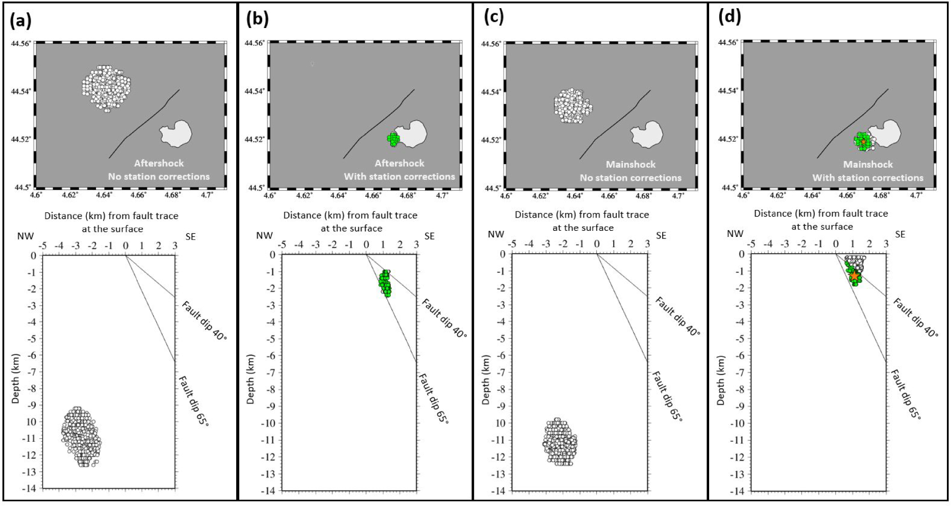
Hypocenter solutions after relocation of the mainshock with station corrections are distributed in depth between 0.2 km (the minimum allowed in the inversion) and 1.9 km. If we retain only solutions compatible with a fault dip between 40° and 65°, the average hypocenter is at 44.5188 N, 4.6694 E, and 1.3 km depth (orange star in Figure 4d).
4. Relocation of the mainshock using a dual velocity model
As mentioned in the introduction, a systematic location bias may rise from a lateral contrast in velocity. We explore this possibility through the strategy illustrated in Figure 5. Again, we used the well-located aftershock as a reference event. However, in this section, it is used to identify a geographical separation among the travel time residuals at station set “shared”, which in turn motivates the search of two distinct 1D velocity models geographically separated. We do not consider station corrections in that case.
The first step is the same as in the previous section, the aftershock is located with station set “post” using the GRIDSIMODLOC approach (step 1 of Figures 2 and 5). However, we do not use the resulting velocity model, previously called optimum local velocity model, in the following steps. On the other hand, the aftershock location obtained with this dense post-seismic network is kept fixed in the following steps.
In step 2, we search for an optimum velocity model at the broader scale of station set “shared”, using the aftershock again. To do that, we use a version of the GRIDSIMODLOC program where the hypocenter can be fixed, so that the sole exploration concerns the velocity model. The velocity model obtained is presented in Figure S3a, Supplementary Material. Then, we analyze how travel time residuals are distributed among the six stations. At stations A192, CRU1, ADHE, and OGDF, P wave residuals are small (<0.15 in absolute value) and S wave residuals are large and positive, ranging from +0.46 at A192 to +1.56 at OGDF. These positive S residuals mean that the observed arrival times are larger than the calculated ones, that is, that the S velocity model is too fast. As a first hint, we can infer that a larger Vp∕Vs ratio should be used for these stations. On the other hand, at stations A184 and BANN, residuals are moderately negative, both for the P and S waves, with values ranging from −0.32 to −0.69. This means that the velocity model is slightly too slow for these two stations. From this simple analysis, a geographical separation emerges, between two subgroups of stations, four of them are located in the SE and the other two in the NW, as illustrated on the top right map of Figure 5.
Strategy followed to search for a velocity contrast that may explain the systematic bias of locations toward the NW. The white dashed line in the upper right map divides the station set “shared” into a NW and a SE subset. On the top left map, the light gray area with a black contour shows the approximate area of the limestone quarry, and the black line is the simplified trace of the mainshock surface breaks.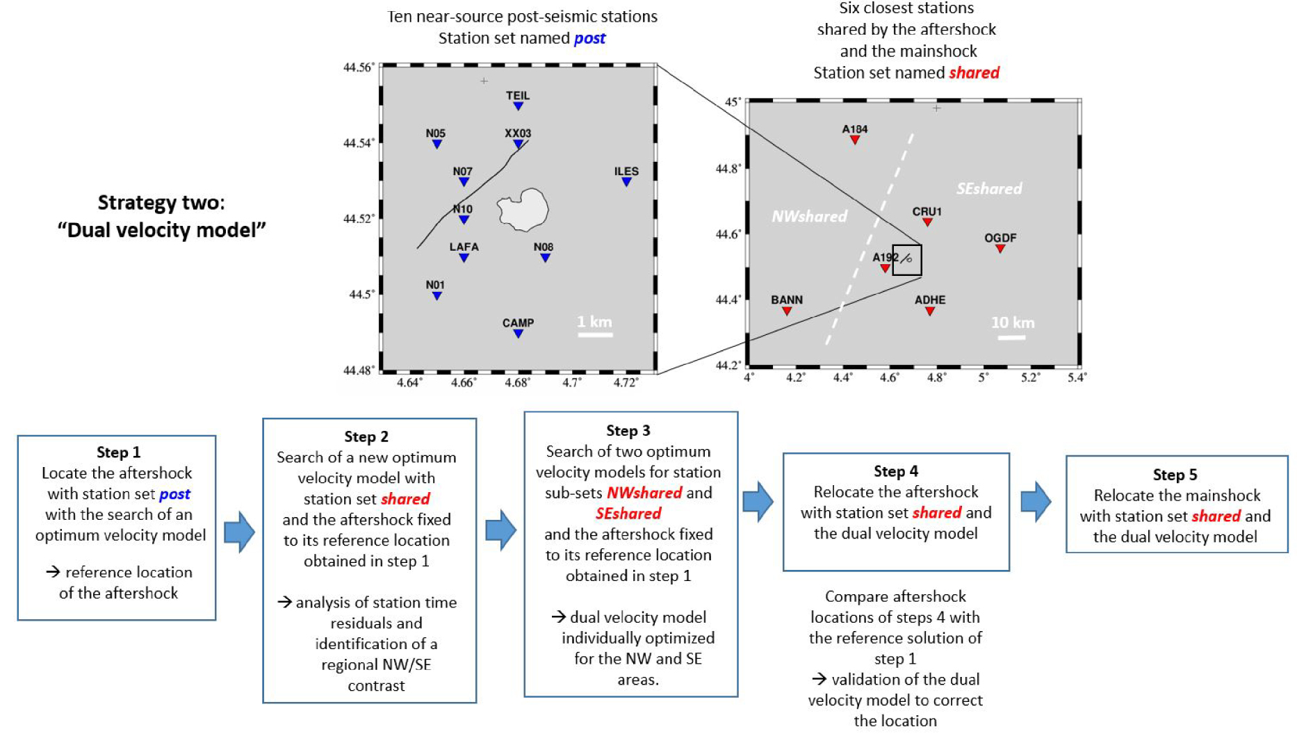
In step 3, we subdivide the dataset of the aftershock in two, corresponding to phase data associated to the “NWshared” and “SEshared” station sets (Figure 5), and perform an exploration of the 1D velocity model for each data set separately, maintaining the hypocenter of step 1 fixed. The two velocity models are presented in Figure S3, Supplementary Material. For the NW area, the P wave velocity at the surface is high, 5.5 km/s, and linearly increases to 7.0 km/s down to the depth of 30 km. The obtained Vp∕Vs ratio (1.69) in the crust is low. For the SE area, the P velocity at the surface is slightly lower, 5 km/s, increasing linearly to reach 7 km/s at 30 km depth. The Vp∕Vs ratio (1.9) is much higher. The main features that could be inferred from the distribution of time residuals in step 2 are effectively retrieved and confirmed by the inversion.
Result of the GRIDSIMODLOC inversion for the aftershock (a) and for the mainshock (b) using the “shared” network of six stations, with the dual velocity model. Top: map view. Bottom: NW–SE cross-section perpendicular to the fault strike. Circles are the best solutions, filled in green when compatible with the main fault dipping between 40° and 65° to the SE. On top maps, the light gray area with a black contour shows the approximate area of the limestone quarry, and the black line is the simplified trace of the mainshock surface breaks. Green solutions are also displayed for the aftershock though it did not necessarily occur on the main fault (see discussion). The orange star in (b) is the average of the green solutions, at 44.5146 N, 4.6739 E, and 2.7 km depth (orange star in Figure 6b).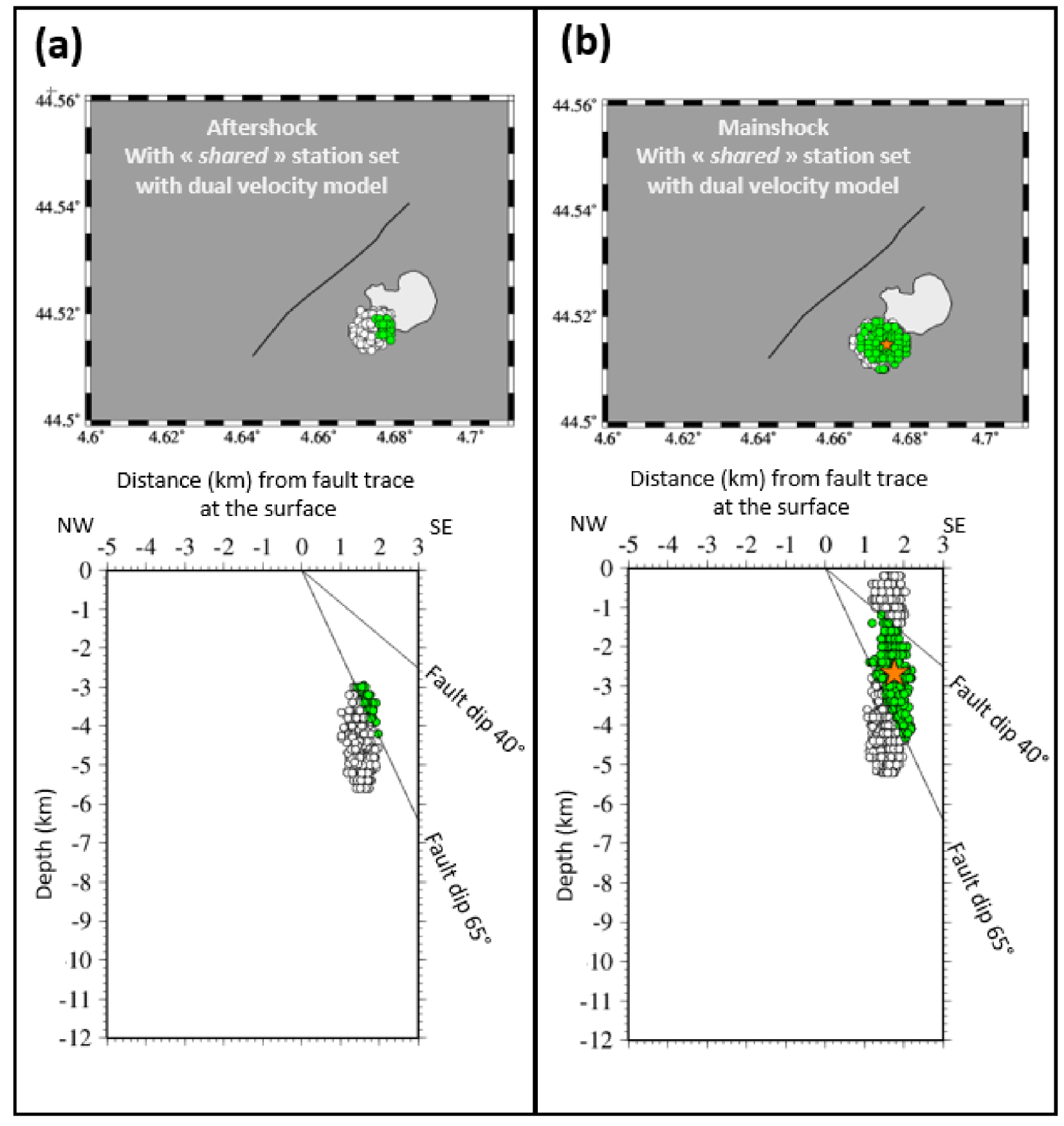
In step 4, we relocate the aftershock using the dual velocity model described above. The result is shown in Figure 6(a). If we compare with Figure 3, corresponding to the reference solution obtained with the dense “post” network, the results are similar, with epicentral solutions shifted a few hundred meters to the SE and hypocentral solutions 2–3 km deeper.
In step 5, we relocate the mainshock using the same dual velocity model. The result is shown in Figure 6(b). If we compare with Figure 4(d), corresponding to the relocation with station corrections, the results are also similar, again with epicentral solutions shifted a few hundred meters to the SE and the hypocenter solutions reaching deeper. The hypocentral solutions are distributed between 0.2 and about 5 km depth. If we retain only solutions compatible with a fault dip between 40° and 65°, the average hypocenter is at 44.5146 N, 4.6739 E, and 2.7 km depth.
The distributions of RMS values as function of the latitude, longitude, and depth corresponding to the different steps 4 and 5 are shown in Figure S4, Supplementary Material.
Overall, the use of the dual velocity model corrects for the mislocation bias which shifted the epicenters several km to the NW of the fault, both for the aftershock and the mainshock, and it locates the hypocenters at much shallower depth.
If we compare the RMS distributions for the master event and dual velocity models (Figures S2d and S4b, Supplementary Material), an overall slightly lower value of RMS is obtained with the master event technique (0.13 versus 0.16), with RMS distributions more peaked. For that reason, our preferred hypocentral determination is that of the master event approach. However, the dual model approach, beyond confirming the overall result of the master event approach, provides velocity models which will be useful to improve waveform modeling, as described in Section 7.
Mainshock relocation relative to a quarry blast. (a) Examples of seismograms of the mainshock and a quarry blast, recorded on four stations (see labels on the left), and their P wave pick ranges (color bands include picking uncertainty). The data are high-pass filtered above 2 Hz. For plotting purposes, we have artificially saturated the signals. Start time is a minute prior to the cataloged event time: 2019-11-11T10:51:45 and 2019-11-08T10:05:27, for the mainshock and blast, respectively. (b) Kernel density plots of relocation results, accounting for the P wave picking uncertainties in map view (left), West–East cross-section (middle), and the cross-section perpendicular to the La Rouvière fault trace. Marginal distributions are plotted on the side and on top. The golden diamond indicates the location of the quarry blasting location; and the yellow star, the mainshock epicenter location determined by the master event approach with station corrections. Quarry border is shown in solid gray line in the map view. Inclined lines on the rightmost graph show the fault dipping 40° and 65° to the SE as in the cross-sections of previous figures.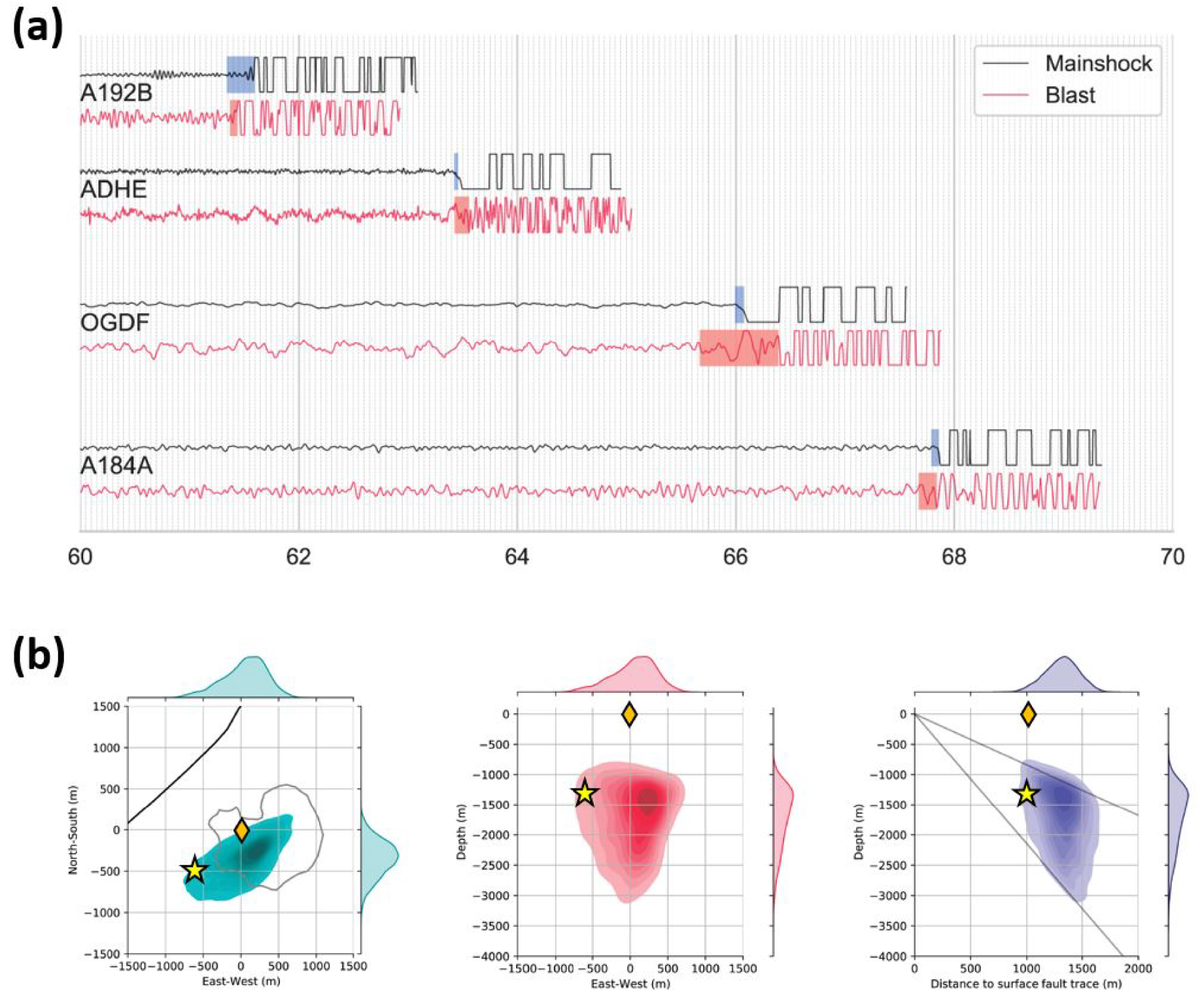
5. Relative location of the mainshock with respect to a quarry blast
In a complementary analysis, we use quarry blast signals (Figure 7a) to relocate the hypocenter and obtain a range of locations that strand over the southwest border of the quarry and overlap with the solutions of our previous approaches. In principle, quarry blasts can be used as ground truth events because their locations (and origin time) are recorded by the quarry operator, and the relative relocation procedure is weakly sensitive to uncertainties in the velocity model outside the source area. In practice, though, quarry blast events come with multiple uncertainties. We referred to the blasting zones reported by the cement company to narrow down the blast location here. Their locations are made available with an uncertainty of ∼150 m in the East–West direction, and much less (<50 m) in the North–South direction. Due to their small equivalent magnitude, their recorded signal-to-noise ratio on regional stations are relatively low, making the picking of their first P arrivals more uncertain than for a regular earthquake. Given their explosive source mechanism with weak S wave radiation, picking of S arrivals is difficult. We quantify here the uncertainties related with exploiting quarry blasts signals to relocate the mainshock hypocenter.
We select the quarry blast of 2019-11-08T10:06:27, which was recorded by seven stations: A192, ADHE, OGDF, A184, #26, #19, #11, and cataloged with a local magnitude (MLv) of 1.7 by the BCSF-RENASS. The same stations also recorded the mainshock and provide a good azimuthal coverage. Station map is given in Supplementary Material, Figure S6. Stations #26, #19, #11 belong to a temporary experiment carried out in the region by the IRSN. We set the blast location as (44.52317N, 4.67744E) at the surface, at the center of the ∼300 m long section of an East–West oriented quarry face indicated as the blasting area by the documentation provided by the Lafarge company. For each station recording, we determine a range of P wave arrival times. Figure 7(a) illustrates our selection of arrival times on four stations. The time picks for all signals are provided in Supplementary Material, Figures S7–S8. Prior to time picking, we resample all the data at the same frequency (250 Hz here, while the initial sampling rate of the selected stations ranges between 100–250 Hz) and applied a 2 Hz high-pass filter. The uniform sampling is applied for convenience of a uniform processing of the different traces. The relative relocation method is based on relating the arrival-time differences between the blast and mainshock signals to the spatial difference between the blasting zone and the hypocenter, as detailed in the Supplementary Material. We use a linearized relation assuming that the source separation is considerably smaller than the source-to-station ray paths, and performed a thorough random sampling of possible solutions accounting for the picking uncertainties and priors on fault geometry.
Figure 7(b) displays the spatial extension of the relocated hypocenters that are compatible with the fault dip uncertainties. The best solution points to a hypocenter depth in the range of 1–1.5 km and is located within the quarry, on its western half. The range of solutions extends beyond the western edge of the quarry and overlaps with the hypocenter locations determined by the previous methods (see discussion). Taking into account the uncertainties in both methods, their results are not inconsistent.
6. Focal mechanism of the mainshock and the aftershock from first motion polarities
We read the P wave first motion polarities at available stations in France and neighboring countries. The maximum distance at which we could determine first motion polarities is 640 km for the mainshock and 100 km for the aftershock. The smaller distance in the latter case is related to the smaller magnitude leading to lower signal-to-noise ratios. Double-couple focal mechanism solutions are explored with the FOCMEC program [Snoke 2003; http://ds.iris.edu/pub/programs/focmec/].
The focal mechanism for the mainshock is determined at the average hypocenter found with the master event technique with station corrections (44.5188 N, 4.6694 E, and 1.3 km depth, step 5 of Figure 2, orange star in Figure 4d) using the optimum local velocity model. Despite the large number of first motion data (114), the focal mechanism can vary significantly as illustrated in Figure 8. All three solutions displayed have three unexplained polarity data, over a total of 114. Two of those are located close to the nodal planes (green circles, Figure 8), and are not a matter of concern. One wrong polarity is farther away from the nodal plane, corresponding to station A180 (red circle, Figure 8). However, this particular station is located approximately at the crossover distance where subtle modifications in the velocity model can change a Moho refracted path to a direct one much closer to a nodal plane. Overall, first motion data are very consistent with the focal solutions.
Three representative solutions for the mainshock focal mechanism determined from first motions of the P wave. Station names are indicated, connected to the corresponding polarity data with a straight line. Green or red open circle: polarity of opposite sign with respect to its respective quadrant, either close to a nodal plane (green), or far from it (red, A180). Station names may be truncated if they contain more than four letters.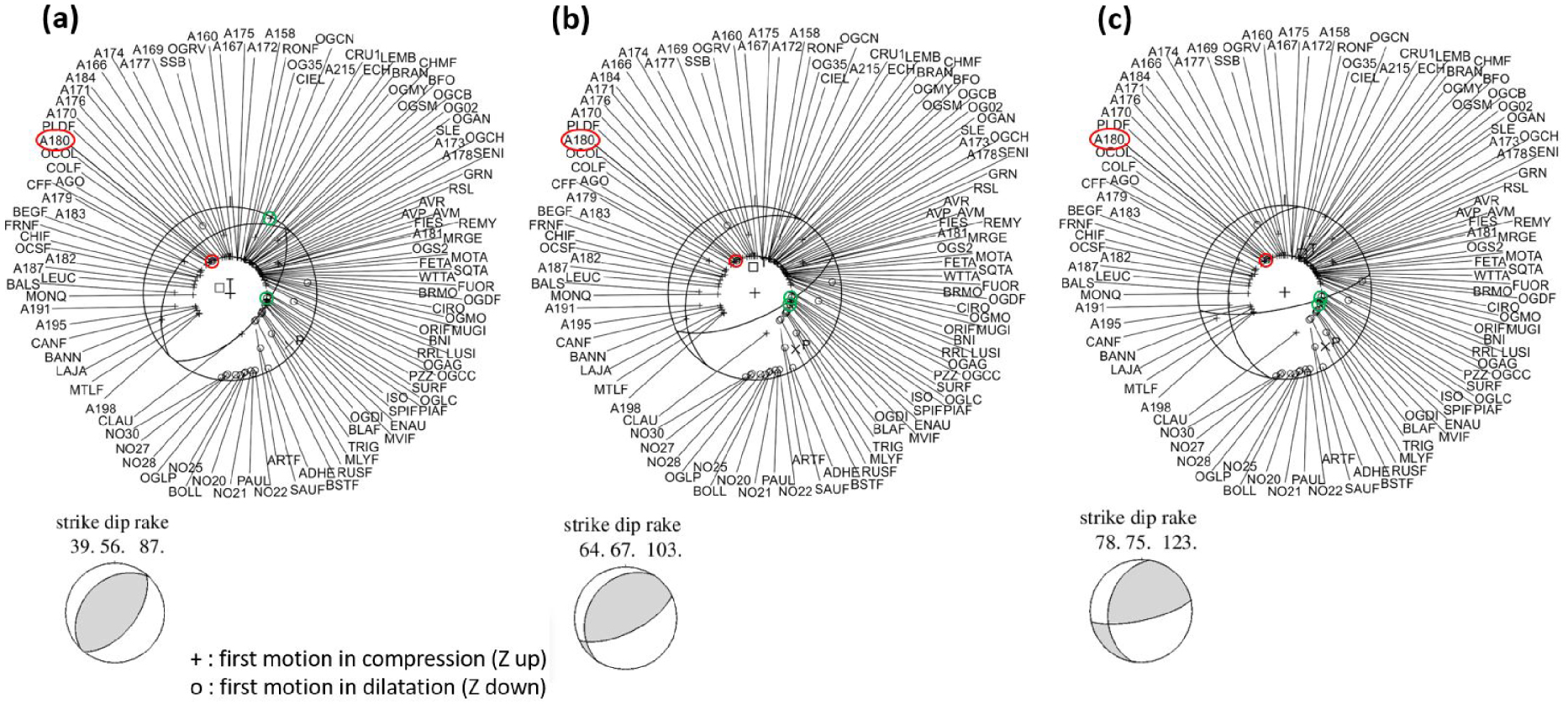
In Figure 8, the strike, dip, and rake angles are indicated for the SE-dipping nodal plane corresponding to the rupture plane. The almost purely reverse solution (a) is the most consistent with the known geometry of the La Rouvière Fault, on which the Le Teil mainshock is reported to have occurred [Cornou et al. 2021; Ritz et al. 2020]. From solutions (b) and (c), the SE-dipping nodal plane rotates toward a more EW orientation, with an increasing right-lateral component.
The focal mechanism for the aftershock is determined at the average hypocenter found with the dense post-seismic network (44.5198 N, 4.6713 E, and 1.8 km depth, Figure 3) using the optimum local velocity model (step 1 of Figure 2). Despite a smaller number of first motion data (48), their shorter distances help to better sample the focal sphere. Consequently, the focal mechanism is very well constrained, within a few degrees (Figure 9). One polarity, from station ILES, shows a clear incompatibility with the focal mechanism. It remains unexplained since the P wave first motion is clear and exhibits a coherent pattern on the N, E, and Z component with respect to the azimuth of the station. On the other hand, station A180 whose polarity is wrong in relation to the main shock focal mechanism is correct here, supporting the explanation of the exchange between a direct path and a refracted path in the case of the main shock. The solution essentially exhibits reverse faulting, with a moderate left-lateral component for the SE-dipping nodal plane. The focal mechanism of the aftershock closely resembles the solution (a) in Figure 8 for the mainshock.
Focal mechanism of the 23 November 2019 aftershock determined from first motion of the P wave. Station names are indicated, connected to the corresponding polarity data with a straight line. Green or red open circle: polarity of opposite sign with respect to its quadrant, either close to a nodal plane (green), or far from it (red). Station names may be truncated if they contain more than four letters.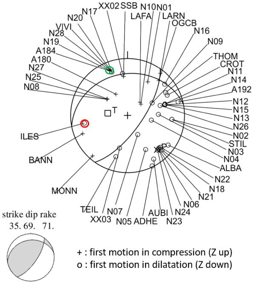
7. Focal mechanism of the mainshock by waveform inversion
The double-couple point source focal mechanism of the mainshock is first explored by waveform inversion with a revised version of the FMNEAR method [Delouis 2014], using 14 stations among the nearest regional unsaturated broadband and strong-motion records (Figure 10a). The inversion is carried out using a combination of grid search and simulated annealing, allowing an extensive exploration of the parameter space. The criterion to select solutions is the minimization of a normalized RMS misfit function of the waveforms. The inversion is repeated for various fixed values of source depth, in order to finely explore this parameter. A first inversion following this approach has been published in Ritz et al. [2020]. Here, we adapt the inversion in three different directions: (1) we use the average hypocenter found with the master event technique and station corrections (this study, 44.5188 N, 4.6694 E, and 1.3 km depth); (2) we use a dual velocity model, differentiated for the NW and SE stations, adapted from the dual velocity model found in Section 4; and (3) we invert the waveforms at higher frequency.
Synthetic seismograms in FMNEAR are computed using the discrete wavenumber method of Bouchon [1981] designed for 1D layered velocity models. For routine and near real time determinations (e.g., http://sismoazur.oca.eu/focal_mechanism_emsc), FMNEAR works with a standard model which was first introduced to model the 2009 L’Aquila earthquake and which is described in the electronic supplement of Delouis [2014]. We started with an inversion with this standard model, but data fitting could be improved by carrying the inversion with two distinct 1D velocity models for the NW and SE areas, incorporating four layers representing the crust and following closely the parameters of the dual velocity linear gradient model found in Section 4 (models b and c of Figure S3). With this dual model, waveform fitting is significantly improved. From the standard model to the dual model, the RMS misfit function decreases from 0.59 to 0.416, corresponding to an increase of the variance reduction (VR) from 65% to 83% [VR = (1 − RMS2) × 100]. Velocity models used with FMNEAR are detailed in Table S2, Supplementary Material.
Waveforms are filtered using a causal Butterworth bandpass filter. The frequency band varies from one station to another, depending on the signal/noise ratio. Most stations are filtered between 0.05 and 0.15 Hz, but the details can be found in Table S3, Supplementary Material.
The complete final result is shown in Figure 10. The best solution corresponds to (strike, dip, rake) = (48, 45, 88), a seismic moment M0 = 2.47 × 10²³ dyne⋅cm, meaning a moment magnitude Mw 4.9. The average Mw calculated on the different explored solutions weighted by the inverse of their respective RMS is 4.8 with a standard deviation of 0.2.
CRU1, BANN, and OGLP have a slightly higher level of misfit (Figure 10c), which may be related to the fact that short-range stations are downweighted in the inversion to compensate for their larger amplitudes in the RMS calculation and to account for the fact that they are more sensitive to small errors in the epicenter position.
Result of the FMNEAR waveform inversion with the dual velocity model. (a) Map with stations used (green triangles) and the focal mechanism corresponding to the best solution found. The white dashed line separates the area into the NW and SE subareas associated with different velocity models (b) Plot of focal mechanism solutions (in red) in an RMS versus depth graph. The best solution is drawn at a larger scale in gray with its strike, dip, and rake parameters. (c) Waveform fit, in displacement (cm) bandpass filtered (see text). Observed records are in gray and computed in red. For each station the three components are displayed (N, E, Z), and “vel” or “acc” means that the original record was in velocity (broadband) or in acceleration (strong motion), respectively.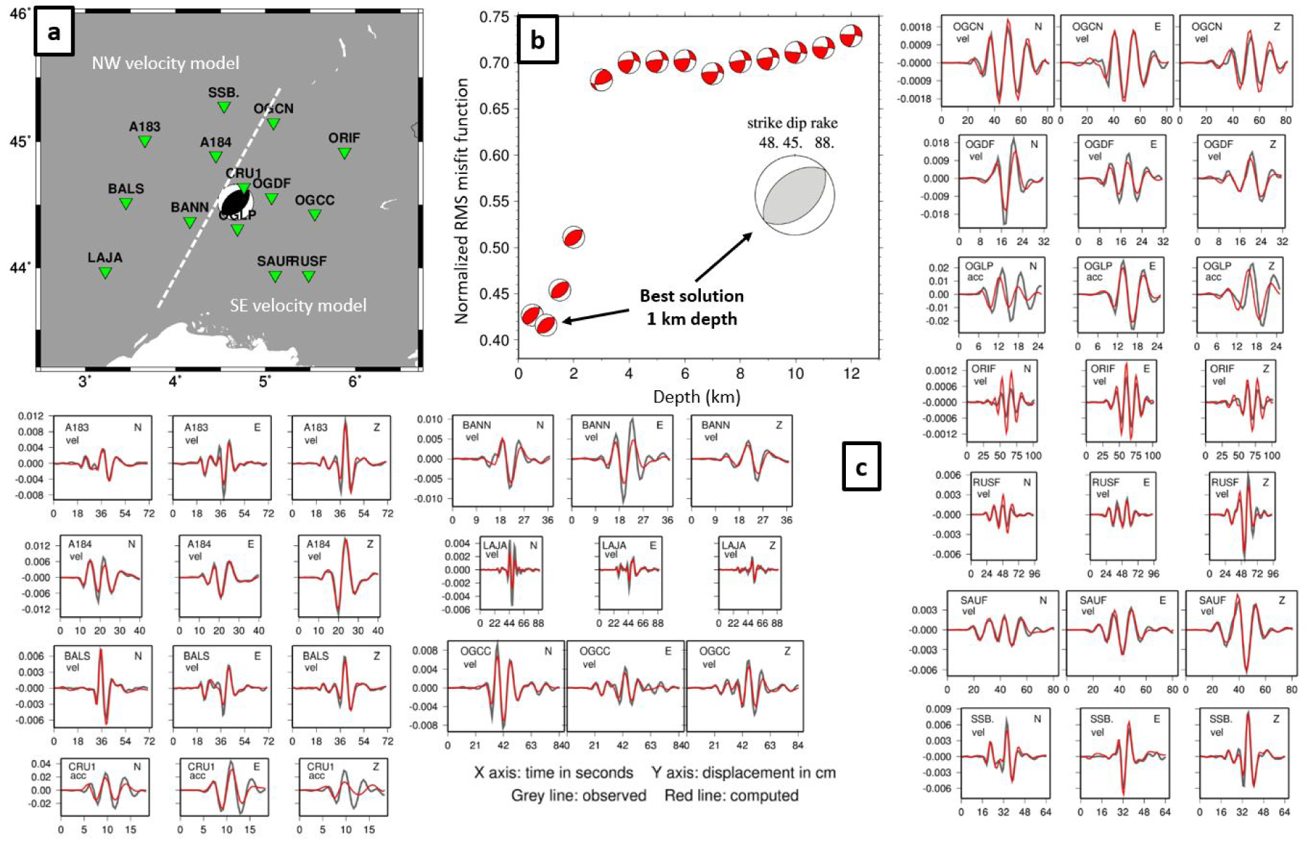
In the nonlinear inversion in the FMNEAR approach, all explored solutions for the focal mechanism are stored with their respective RMS misfit function, allowing a posteriori analysis of the uniqueness or variability of the solution. Solutions with the lowest RMS values, that is, the largest values of variance reduction (VR), above 79%, exhibit all reverse faulting with nodal planes oriented NE–SW (Figure 11). However, we observe that the dip of the SE-dipping nodal plane corresponding to the rupture plane varies between 40° and 60°. Note also that the azimuth of the SE-dipping plane, may move to a more EW orientation (strike 65), in a similar way as the first motion solution (Figure 8).
Extract from the stored solutions found by the FMNEAR waveform inversion with the dual velocity model. Around each beach ball are indicated the corresponding values of the strike, dip, rake parameters (above) and the RMS and variance reduction (VR) (below). The solution on the left is the best one, corresponding to Figure 10, and the next ones moving to the right are ordered by decreasing value of VR, remaining larger or equal to 80%.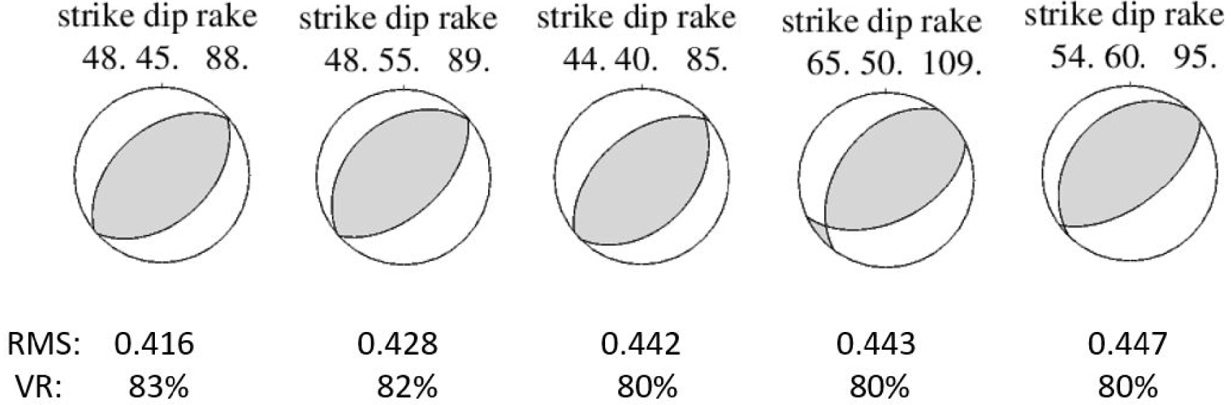
Variation of the variance reduction (VR) as a function of the strike, dip, and rake parameters of the focal mechanism with the TDMT approach. Note the large plateau with VR values comprised between 75 and 82% for dip values ranging between 20° and 70°.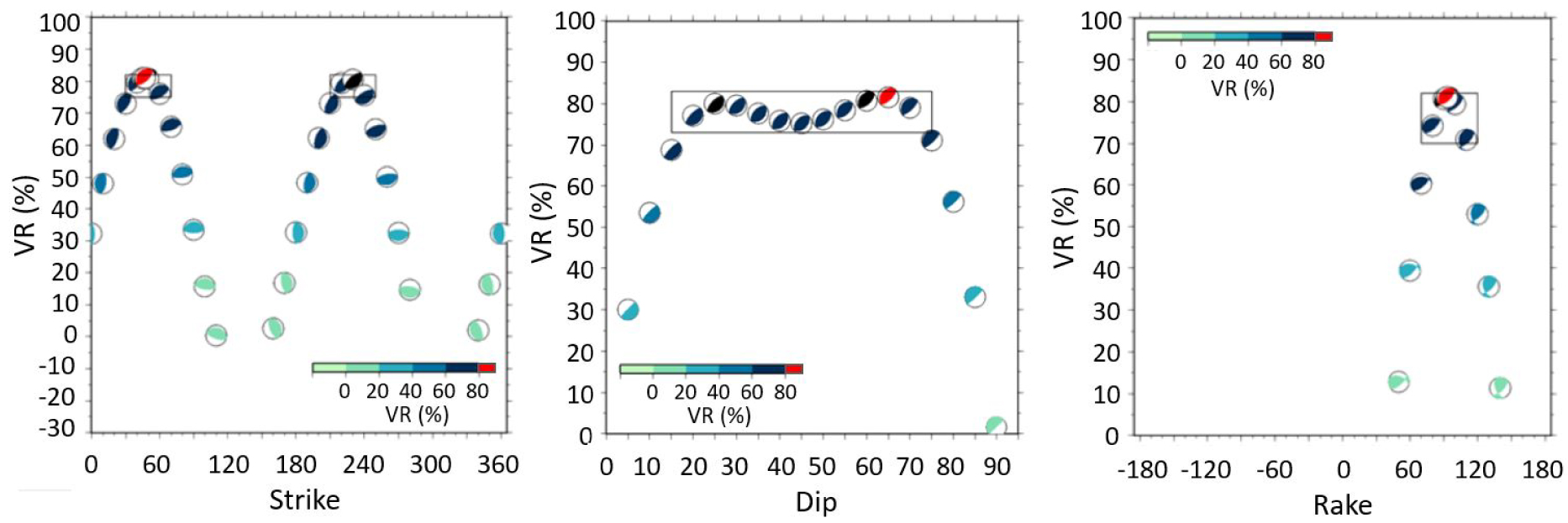
Interestingly, the focal mechanism solution (reverse faulting with SE and NW-dipping nodal planes) and optimal depth (∼1 km) are stable for a wide range of velocity models. We test a number of different velocity models, all resulting in similar solutions. Basically, the waveform misfit function varies depending on the model, but the source parameters remain similar. In some cases, best depth was found at 0.5 km instead of 1 km. On the other hand, the dip value of the SE-dipping nodal plane of the best solutions varies between 40° and 60°.
To further assess the robustness and variability of the source parameters, we include in the present study the result of a waveform inversion based on a different approach, namely time domain seismic moment tensor (TDMT) [Dreger 2003], relying on a largely distinct set of stations, a different filtering band, and a specific velocity model. TDMT determines for a given point source, using a least-square inversion scheme, the deviatoric moment tensor (MT), which can be decomposed into the sum of a double-couple (DC) and a compensated linear vector dipole (CLVD) tensors. The preferred solution from the TDMT inversion is shown in Figure S5 of the Supplementary Material [Vallage et al. 2021]. Waveforms are filtered with a causal Butterworth bandpass filter between 0.03 and 0.08 Hz. Green’s functions are calculated with the velocity model (Table S4, Supplementary Material) used for routine determinations by the CEA/LDG in metropolitan France [Duverger et al. 2021]. The preferred TDMT solution corresponds to a mostly DC seismic reverse source with the same orientation as found by the FMNEAR approach, but with a steeper SE-dipping nodal plane (strike, dip, rake) = (45, 65, 93), and the same preferred depth of 1 km (Figure S5, Supplementary Material). Variance reduction (VR) is similar, 82%, whereas the moment magnitude is slightly lower, Mw 4.8, compared to FMNEAR.
To further investigate the influence of the focal mechanism parameters in more detail, the TDMT algorithm was run for evenly spaced discrete values of the individual parameter strike, dip, and rake, while the other two parameters were kept fixed according to their optimal value found previously (Figure 12). While the strike and rake parameters are well constrained (strike has two optimum values due to the ±180° equivalence in azimuth), the dip angle is clearly and poorly constrained between 20° and 70°. To a lesser extent, Figure 11 shows also that the dip angle is less well constrained by the FMNEAR inversion. Such a large uncertainty on the dip parameters by waveform inversion is not common case and is discussed in the next section.
8. Discussion–Conclusion
8.1. Reference location for the aftershock
Using ten post-seismic stations well-distributed around the rupture zone and with epicentral distances smaller than 5 km, we obtained a reference average location for the aftershock: 44.5198 N, 4.6713 E, and 1.8 km depth. The uncertainty can be estimated at ±500 m horizontally and in depth (Figure 3). With such a dense and nearby network, the hypocenter is expected to be much less sensitive to the velocity model than with farther distance stations. In our approach, we simultaneously determined the aftershock hypocenter and an optimal local 1D linear gradient velocity model. A different local 1D velocity model has been determined by Cornou et al. [2021] and Causse et al. [2021] based on a beamforming method using the seismic noise recorded by the post-seismic stations installed in the fault vicinity. The refined model published in Causse et al. [2021] exhibits an inversion of the P and S velocities, which are divided by a factor of ∼3, at 1.2 km depth. This model is expected to reflect the Earth structure in the epicentral area (epicentral distance <10 km). We have built an alternative velocity model comprising several layers of linear velocity gradient to approximate the model from Causse et al. [2021], with a negative gradient between 800 and 1200 m to represent the velocity inversion. Using this model with the ten stations of the post-seismic network, we obtain hypocenter solutions undiscernible from those found with our optimum local velocity model presented in Figure 3.
8.2. A bias of location satisfactorily corrected
When located with the more distant stations shared with the mainshock, without station corrections and with a single velocity model, the aftershock is shifted several kilometers to the NW on the wrong side of the fault and its hypocenter is shifted several kilometers deeper. The same kind of bias is observed in the location of the mainshock, explaining why the early epicenters determined with the permanent stations were also shifted to the NW side of the fault.
We showed that this bias in location can be corrected either by using a master event technique through station corrections, or by using an adapted velocity model separated in the NW and SE subregions. Station corrections allowed for a more accurate correction of the aftershock hypocenter than the dual velocity model (comparison between Figure 3, which is the reference, and Figures 4b and 6a). Accordingly, we prefer the relocation of the mainshock obtained with the station corrections, that is, by the master event technique, at 44.5188 N, 4.6694 E, and 1.3 km depth, over that obtained with the dual velocity model. The relative location with respect to a quarry blast is another way by which we could locate the mainshock hypocenter on the correct side of the fault. All three approaches provide shallow hypocentral depths compatible with the geometry of the fault plane inferred from independent studies.
8.3. Comparison of epicenters and area of compatibility for the mainshock
Figure 13 compares the epicenters of the aftershock obtained using the dense post-seismic network with the relocated mainshock epicenters resulting from the master event approach, from the dual velocity model, and from the relative location with respect to the quarry blast. Considering the uncertainty areas, a zone of overlapping can be found for the mainshock (purple shaded area in Figure 13).
Map showing the four epicenters located in this study. The green smaller star is the average epicenter of the 23 November aftershock (44.5198 N, 4.6713 E, and 1.8 km depth). Area of uncertainty is not shown. The red star is the average epicenter of the mainshock (44.5188 N, 4.6694 E, and 1.3 km depth) relocated using the aftershock as a master event, with its uncertainty area delimited by the red dashed curve (from Figure 4d). The blue star is the average epicenter of the Le Teil mainshock (44.5146 N, 4.6739 E, and 2.7 km depth) relocated using the dual velocity, with its uncertainty area delimited by the blue curve (from Figure 6b). In both cases, the dashed line of uncertainty surrounds solutions compatible with the fault geometry and whose RMS is lower than the chosen threshold. The orange star is the relocation of the mainshock relatively to the quarry blast, with the acceptable uncertainty area delimited by the orange dashed curve (from Figure 7b). The purple shaded area is the intersection of the three uncertainty areas for the mainshock epicenter. Heavy black line: simplified trace of surface breaks. Thin closed black curve: approximate contour of the limestone quarry. Background map from the French Geoportal, IGN, https://www.geoportail.gouv.fr/carte.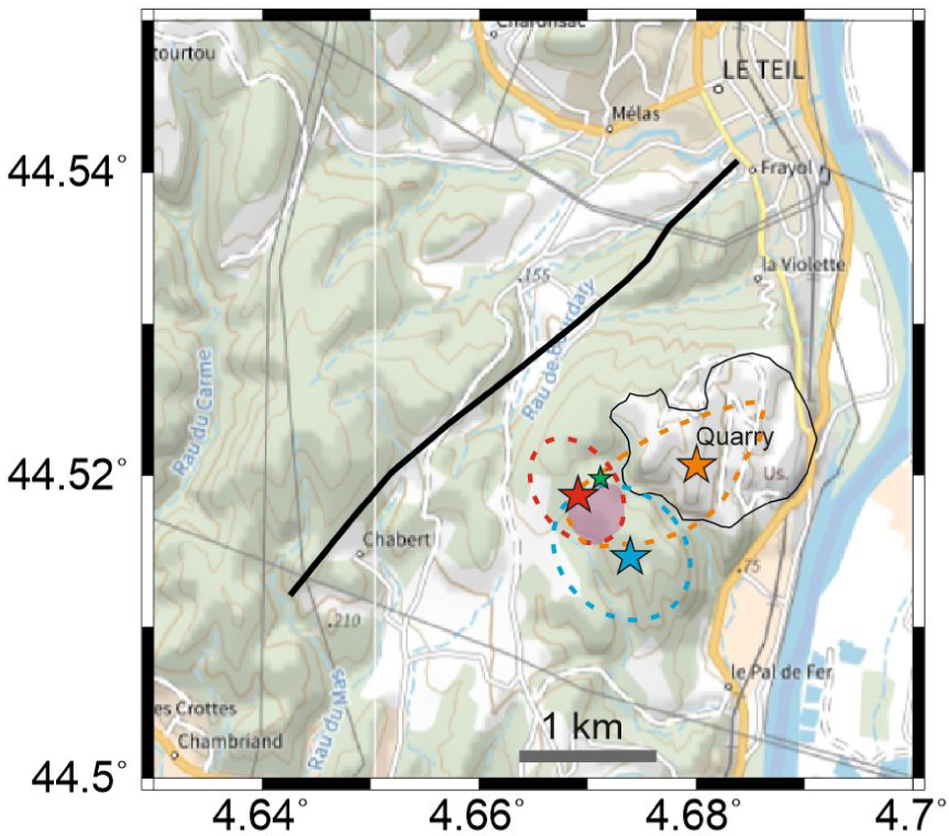
8.4. Mainshock hypocentral depth
We observe a convergence around 1 ± 0.5 km for the depth of the mainshock hypocenter obtained from the relocation with the master event approach (Figure 4d) and from the waveform inversions (Figures 10 and S5, Supplementary Material). Solutions from the relative location with respect to the quarry blast are compatible with this depth interval (Figure 7b). The dual velocity model approach results in a deeper, 2.7 km depth, average hypocenter but with a large uncertainty not preventing a shallower depth (Figure 6b). We retain 1 ± 0.5 km as the most likely depth range for the mainshock.
8.5. Position of the mainshock hypocenter with respect to the rupture area
Whether considering the average solution from the master event method (red star in Figure 13), or the area of compatibility with the alternative approaches (purple shaded are in Figure 13), the mainshock hypocenter is approximately located in the middle of the rupture area constrained by the along fault strike extent of surface breaks [Ritz et al. 2020] and by the InSAR data and derived slip model [Ritz et al. 2020; Cornou et al. 2021]. This observation is coherent with the bilateral character of the rupture found by analyses of the azimuthal distribution of the apparent duration of the rupture by De Novellis et al. [2020] and Causse et al. [2021]. Furthermore, our relocated epicenter (red star in Figure 13) is almost indiscernible from the first subevent identified by Mordret et al. [2020] by analyzing the coherency of high-frequency waveforms at two neighboring far-field stations.
8.6. The dual velocity model reflected in the Geology
The strategy of the dual velocity model in Section 4 can be considered as a degraded version of the master event approach with station corrections. Instead of correcting individually each station, we correct them by group (NW or SE), through the two separated velocity models. However, the resulting dual velocity model (Table S2, Supplementary Material) proved to be useful at a broader scale for the waveform inversion, and it points to a strong and simple velocity contrast between a faster NW and a slower SE domain. The SE domain is characterized by a particularly high Vp∕Vs ratio (1.9). We tested additional models and verified that a Vp∕Vs ratio of 1.8 to 2.0 is required to model properly the S waveforms at the stations of SE France, especially when the low-pass filter frequency used in the waveforms processing is increased. As illustrated by Figure 14, the NW and SE domains used in the waveform inversion (see Figure 10a) correspond to very different geological domains. To the NW, the older, mainly Paleozoic, crystalline and metamorphic basement rocks of the Massif Central dominate largely. To the SE, we enter in the subalpine domain with a thick and deformed secondary and tertiary sedimentary cover. Indeed, the boundary between the two domains corresponds to the NE–SW trending Cévennes Fault System which is a major structural boundary. The preliminary 3D velocity model for metropolitan France by Arroucau [2020] also shows a clear contrast between the two domains, with higher P and S velocities in the upper crust in the Massif Central than further east, as does our dual velocity model (Table S2, Supplementary Material).
To better illustrate the need of a high Vp∕Vs ratio in the SE, we compare the waveform fit at stations OGDF, OGCC, and OGCN located in the SE domain, when the SE and NW velocity models are exchanged for these stations (Figure 15). The same 14 stations as before are included in the FMNEAR inversion, with the same hypocenter. A clear decrease in the waveform fit is observed at OGDF and OGCC, and less obvious but noticeable at station OGCN which is situated near the border between the two domains (Figure 14).
Seismic stations (green triangles with station name) used in the FMNEAR waveform inversion overlaid on the geological map (BRGM, Bureau de Recherches Géologiques et Minières imported from the French geoportal, https://www.geoportail.gouv.fr/carte). Station names are in black or white, depending on the background color, for better visibility. Red colors on the geological map correspond essentially to the Paleozoic crystalline rocks. Light blue, light green, and yellow correspond to Jurassic, Cretaceous, and tertiary sediments, respectively. The black dashed line separates the NW and SE subareas. The epicenter of the Le Teil mainshock is indicated by the orange star.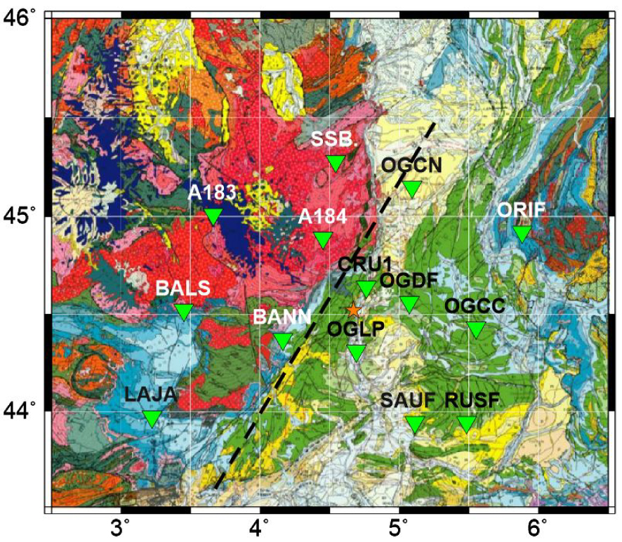
Comparison of waveform modeling at three selected stations of the SE domain, OGDF, OGCC, and OGCN, by modifying the velocity model for those three stations only. They are modeled with the SE velocity model on the left (same as Figure 10) and with the NW velocity model on the right. Waveform in displacement (cm) bandpass filtered (see text). Observed records are in gray and computed in red. For each station, the three components are displayed (N, E, Z), and “vel” means that the original record was in velocity (broadband).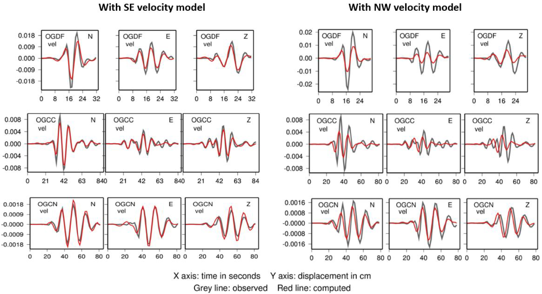
We could also consider a regionalization of the velocity model into three zones, incorporating a third velocity model corresponding to the Cevennes fault system (CFS) zone. Indeed, we observe that stations CRU1 and A192 (Figure 2 top right), closest to the fault zone and the epicenter, have smaller time residuals than the other stations (Table S1). However, these smaller residuals can also be explained by the fact that the difference between the model and real Earth travel times, that is, the residual, is expected to increase with hypocentral distance.
8.7. Source parameters and the La Rouvière fault
The surface trace of the ruptured fault as mapped by the InSAR data and delineated by the 4.5 km long surface breaks in the field [Cornou et al. 2021; Ritz et al. 2020] has an average strike comprised between 40° to 45°. Field observations of the La Rouvière fault scarp indicate that the fault is dipping from 45° to 60° SE at the surface [Ritz et al. 2020]. Modeling of the coseismic InSAR data has been performed with a fault dipping 50° to 60° SE, from the surface to a depth of about 1 km [Delouis et al. 2019; Cornou et al. 2021; De Novellis et al. 2020]. The various solutions for the focal mechanism resulting from the waveform inversions (Figures 11 and 12) are in good agreement with those parameters for the SE-dipping rupture plane, although they exhibit a certain degree of indetermination, especially for the dip angle. The focal mechanism from the first motion data (Figure 8) displays a significant variation in the strike of the SE-dipping plane. Solutions b and c in Figure 8 are clearly incompatible with the fault strike derived from field and InSAR observations, but the solution compatible with the fault orientation (Figure 8a) indicates a dip of 56° SE.
Unfortunately, waveform inversions do not really help in constraining the fault dip of the Le Teil earthquake at depth. This lack of constraint may be related to the very shallow depth of the earthquake. The existence of a trade-off between fault dip and the seismic moment M0 in the case of shallow dip-slip earthquakes is well documented for methods relying on long period surface waves [e.g., Kanamori and Given 1981]. However, our approach here inverts for the full waveforms, including the body waves. One way to address the question of indetermination of the dip angle in the present case would be to carry out synthetic tests, but this is beyond the scope of the present paper.
On the other hand, the variability in the dip angle as seen through waveform inversions could reflect a variation of the dip angle of the rupture plane with depth. The La Rouvière fault is an ancient Oligocene normal fault belonging to the northern part of the CFS whose kinematics has been inverted, and these ancient normal faults have typically a listric geometry [Ritz et al. 2020]. In the full waveform inversions presented in this study, the rupture is approximated by a point source averaging the real rupture properties. Depending on which part of the waveforms is best modeled, the point source may reflect slightly different parts of the rupture from one solution to another. If this is occurring, we can envision a listric rupture plane whose dip angle varies from about 60° at the surface to 30°–40° at about 1 km depth. However, the first motion focal mechanism, reflecting the rupture geometry at rupture initiation (hypocenter) at about 1 km depth favors a steep dip angle (56°). This last observation is in favor of a straight fault plane, from the surface down to 1–1.5 km depth, with a rather constant dip between 50° and 60°.
Regarding the strike-slip component, solutions for the focal mechanism compatible with the rupture strike (∼45°) may display small right- or left-lateral components of motion, meaning that it is probably too small to be resolved. We conclude that the mainshock involved essentially pure reverse faulting.
Regarding the aftershock (Figure 3), its location and focal mechanism (Figure 9) are compatible with the La Rouvière fault that ruptured during the mainshock [Ritz et al. 2020], although we cannot completely rule out that this event occurred on a secondary fault with similar geometry. The moderate but clear left-lateral component of motion on the SE-dipping nodal plane of the aftershock could be related to the small counterclockwise rotation of its azimuth relative to that of the main rupture plane, or to a local perturbation of the regional stress tensor produced by the main rupture.
The updated mainshock hypocenter contributes to the study of the possible triggering of the Le Teil earthquake by the cement quarry that lies above the fault. Coulomb stresses on the La Rouvière fault due to rock extraction from the quarry were estimated by Delouis et al. [2019], De Novellis et al. [2021], and Liang and Ampuero [2020]. Our updated hypocentral area is located in an area of significantly increased Coulomb stress, exceeding 100 kPa, which is in the range of the values that were previously reported to have triggered earthquakes in various contexts [McGarr et al. 2002 and references therein; Harris 1998, and references therein; Ziv and Rubin 2000].
The hypocentral depth near the base of the mainshock rupture area is consistent with the hypothesis that the characteristics of the earthquake are controlled by lithological layering [Causse et al. 2021]. Below the hypocentral depth, the fault cuts through marly rock layers, which could give it a frictionally stable behavior that promotes fault creep [e.g., Gratier et al. 2013]. More precisely, the fault cuts through the Valanginian formation which is dominated by soft marls [Causse et al. 2021]. If the deeper portion of the fault creeps aseismically, without significant stress accumulation, its low stress could have slowed down and ultimately stopped the mainshock rupture. Moreover, deeper fault creep prior to the mainshock would tend to concentrate stresses right above the creeping portion. Such a stress concentration, in turn, can explain why the hypocenter is located near the base of the rupture. Indeed, earthquake nucleation typically occurs near boundaries between coupled and uncoupled fault areas in numerical models [e.g., Lapusta and Rice 2003] and in some large-scale faults [e.g., Ader et al. 2012; Avouac et al. 2015].
Acknowledgments
We are grateful to the Réseau Sismologique et géodésique Français (RESIF) (http://dx.doi.org/10.15778/RESIF.FR, http://dx.doi.org/10.15778/RESIF.RA) for making seismological records available. Same for the French Global Network of broadband seismic stations (GEOSCOPE) (http://dx.doi.org/10.18715/GEOSCOPE.G). A special thanks to Anne Paul, who facilitated the access to records of the AlpArray temporary network (http://dx.doi.org/10.12686/alparray/z3_2015). We are also grateful to the Electricité de France (EDF) for providing access to seismological records in the vicinity of the Le Teil earthquake. Part of the research that led to this publication is based on seismic data acquired by the Institut de radioprotection et de sûreté nucléaire (IRSN) in November 2019. We are grateful to the LafargeHolcim ciments company, who gave us access to the location of the quarry blast used in this study. Finally, we are thankful to the two anonymous reviewers, who helped us in improving the manuscript.