


 CC-BY 4.0
1. Introduction
Benthic nutrient fluxes in coastal ecosystems, especially in shallow environments, are impacted by both biotic and abiotic processes in the sediment [Boynton et al. 2018; Santschi et al. 1990; Ståhlberg et al. 2006]. One of the major processes of the early diagenesis of sediment is the microbial degradation of sedimentary organic matter (SOM), producing ammonium () and phosphate () and the consequent fluxes of N and P at the sediment–water interface [Flint and Kamykowski 1984; Sigmon and Cahoon 1997; Anderson et al. 2003].
The degradation of SOM, and consequently N and P fluxes, depends on its quantity and composition but also on external factors such as physico-chemical characteristics of the sediments (porosity, grain-size and mineralogy), temperature and availability of electron acceptors as well as microbial and macrobenthic activities and diversities [Arndt et al. 2013; Freitas et al. 2021; LaRowe et al. 2020]. However, the relative significance of these factors remains poorly quantified however [Freitas et al. 2021], preventing the prediction of the effect of climate and environmental changes as well as the development of mitigation strategies.
Although the amount of SOM has been reported as an important driver of mineralization activity in coastal areas [Sloth et al. 1995; Mesnage et al. 2007], the composition of SOM has also been shown to play a key role in benthic nutrient cycling [Andrieux-Loyer et al. 2014; Albert et al. 2021]. The composition of SOM in coastal areas is tightly linked to its origin and is the result of a large diversity of allochthonous and autochthonous primary producers (such as phytoplankton, benthic macroalgae, microphytobenthos, seagrasses andwoody plants), as well as anthropogenic OM [Bianchi and Bauer 2011, and references therein]. Among natural sources of OM, the pathways from sources to sediments and the probability of early biodegradation differ greatly between autochthonous and allochthonous OM. Allochtonous OM has undergone transport from sources to sediments and along its transfer has possibly been subject to biodegradation and can be protected by interactions with mineral surfaces, in contrast to autochthonous OM which only experiences vertical transport and settling. Consequently, the latter would be richer in labile molecules, which could explain the higher reactivity in sediments following phytoplanktonic blooms [Franzo et al. 2019; Grenz et al. 2000]. Moreover, anthropogenic sources of OM from sewage and soil fertilization by agricultural amendments may also drive sedimentary P cycling [Ait Ballagh et al. 2020; Khalil et al. 2018]. However, the respective role of allochtonous versus autochthonous and anthropogenic versus natural OM on the biodegradability of SOM and the diffusive and advective benthic nutrient fluxes remains unclear.
In order to investigate the relationships between the origin of SOM and benthic nutrient fluxes, 200 intertidal mudflat sediments from 12 mudflats along the coastline of Brittany, France were sampled. In this region, marine intertidal mudflats are influenced by river discharges and large tidal fluctuations. Agricultural intensification and the urbanization of watersheds have led to coastal eutrophication, where macroalgal “green tides” occur regularly in spring [Ménesguen et al. 2019; Perrot et al. 2014; Schreyers et al. 2021]. Designing the investigation at the scale of the region allows the investigation of variations in the proportions of natural (marine versus terrestrial) and anthropogenic sources of SOM, while terrestrial plant precursors, land use and sources of anthropogenic pressure remain unchanged. The composition of SOM was studied by a combination of isotopic (δ13C and δ15N values) and lipid (aliphatic hydrocarbons (n-alkanes and hopanes), sterols and stanols, fatty acids, fatty alcohols, and aromatic hydrocarbons including polycyclic aromatic hydrocarbons-PAH) analyses classically used to investigate the sources of SOM [Freese et al. 2008; Volkman et al. 2000]. The ability of sediments to release and fluxes through diffusion were determined using incubations with intact sediment cores under the same ambient experimental conditions (dark, controlled temperature, artificial overlying water) [Louis et al. 2021]. Finally such a dataset allows the use of canonical redundancy analysis (RDA) and variance partitioning in order to explain the spatial variability of the and fluxes as independent parameters related to (i) the variation of the SOM origin (elemental and isotopic ratios, lipid markers) and (ii) the variation of the elemental composition (N, P, C) and physical properties (grain size, porosity) of the sediment [from Louis et al. 2021].
The different analytical techniques will shed light on the composition of the SOM, which will allow the determination of its spatial variability and origin. In combination with statistical analysis this will allow relating quantitatively the impact of the origin of SOM on benthic nutrient fluxes in shallow coastal environments.
2. Materials and methods
2.1. Study sites and sampling
All of the study sites were macrotidal mudflats, located in Brittany, north-western France, and have been described in detail previously [Louis et al. 2021]. In short, 200 sediment samples were collected at low tide at 45 sites and were classified into 12 mudflats (Figure 1) during spring 2019. Sampling sites were divided into three classes: bay, lower estuary and middle estuary according to their distance to the mouth; from 0 to 5 km and from 5 to 15 km, respectively. Sediment cores (10 cm depth) were sampled with PVC tubes (diameter = 6 cm, h = 20 cm) to measure the nutrient benthic fluxes, and another tube (diameter = 9 cm, h = 5 cm) was sampled to characterize the SOM (elemental, isotopic and lipid composition) and physico-chemical parameters (grain size distribution and porosity) in the upper 5 cm layer. Even though the flux measurements were carried out with 10 cm depth sediments, the nutrient fluxes are the result of gradients over the first 2 to 5 cm [Lee and Kim 1990; Akbarzadeh et al. 2018]. In order to capture this reactive zone, the first five cm of the sediment were analyzed for physico-chemical parameters. Elemental composition (total organic C, total N, total, organic and iron oxide bound P), grain-size distribution, porosity and benthic nutrients fluxes were described in a previous paper [Louis et al. 2021], while isotopic and lipid compositions are the new data discussed in this paper.
Location of the mudflats and sampling sites (n = 45) on the Brittany coast. Goulven Bay and Aber Wrac’h are two different mudflats, as are Vannes Estuary and Morbihan Gulf. The sampling sites were divided into three groups according to their geographic locations into “Bay” (pink), “Lower estuary” (green) and “Middle estuary” (blue).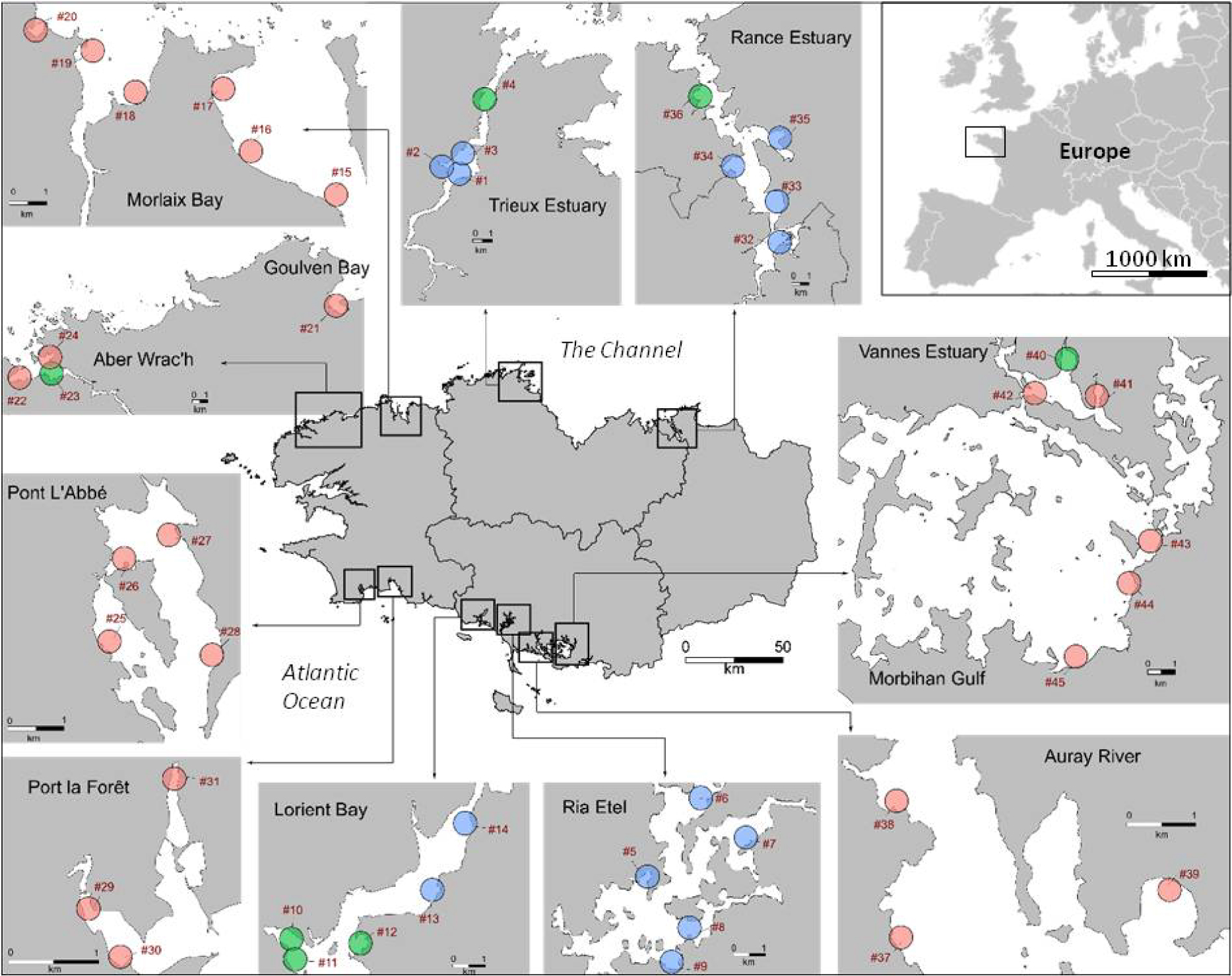
2.2. Isotopic analysis
The carbon and nitrogen isotopic compositions (δ13C and δ15N values) were determined using an element analyzer (FLASH™ EA 2000 IRMS) coupled with an isotopic ratio mass spectrometer (DELTA V™ plus). An aliquot of the 5 cm pooled sample was freeze-dried, crushed and acid-treated with 2N HCl to remove the carbonate and was subsequently rinsed with deionized water. After centrifugation, the carbonate-free sample was dried at 60 °C, and ground before being placed into a tin capsule for stable C isotopic analysis. A second aliquot without an acidification treatment was used for the total nitrogen in bulk OM (TN) and stable N isotopic analysis. All isotopic analyses were performed once and data were expressed in the conventional delta notation relative to the Vienna Pee Dee Belemnite for δ13C values and to atmospheric N2 for δ15N values. Data calibration and determination of the accuracy and reproducibility was carried out using two international standards IAEA-N2 and IAEA-CH-6 and a certified standard IVA33802151 organic-rich sediment. Repeated analysis indicated analytical uncertainty better than ±0.2‰.
2.3. Lipid marker analysis
An aliquot of the 5 cm pooled sample was freeze-dried and crushed. Approximately 30 g of this sample was extracted with approximately 100 mL of dichloromethane using an accelerated solvent extractor (Dionex™ASE™ 200) as per the following conditions, modified from Derrien et al. [2011]: 33 mL cells, 5 min heating at 100 °C and 60 bars, 10 min static phase, completed with 80% flush and 20-s purge with nitrogen. Elemental sulfur was removed from the total lipid fraction by reduction on metallic copper. After evaporation of DCM under a gentle stream of nitrogen, the total lipid extract was fractionated into aliphatic hydrocarbons, aromatic hydrocarbons and polar compounds on a silica column by successive elution with cyclohexane, cyclohexane/dichloromethane (2/1, v/v) and methanol/dichloromethane (1/1, v/v). Polar fractions were analyzed by capillary gas chromatograph-mass spectrometer (QP2010SE GC-MS, Shimadzu) after derivatization using a mixture of N,O-bis(trimethylsilyl) trifuoroacetamide (BSTFA) and trimethylchlorosilane (TMSC) (99/1, v/v), whereas the aliphatic and aromatic fractions were analyzed without further treatment. The injector used was in splitless mode and maintained at a temperature of 310 °C. The chromatographic separation of the three lipid fractions was performed on a SLB-5MS capillary column (length = 60 m, diameter = 0.25 mm, film thickness = 0.25 μm) under the following temperature conditions: 70 °C (held for 1 min) to 130 °C at 15 °C/min, the 130 °C to 300 °C (held for 15 min) at 3 °C/min. The helium flow was maintained at 1 ml/min. The chromatograph was coupled to the mass spectrometer by a transfer line heated at 280 °C. The ionization was performed by electronic impact and analyses were performed in full scan mode. The organic compounds were quantified by using an external calibration adding internal standards in the solutions containing the aliphatic hydrocarbons (internal standards: nC20D42; nC24D50; nC30D62; α-cholestane), aromatic hydrocarbons (internal standards: Naphthalene-D8; Acenaphtene-D10; Phenanthrene-D10; Chrysene-D12; Perylene-D12) and polar compounds (internal standards: nC20D42; nC24D50; nC30D62; α-cholestane) as per Jeanneau et al. [2008].
These analyses provided the total concentration of lipid markers in the dry mass sediment. The results were also expressed as the proportion of each lipid marker as a function of the sum of all lipid compounds quantified in the sediment. Unless otherwise stated, results are presented as the average ± the standard deviation.
2.4. Benthic nutrient fluxes
The and fluxes are previous results described in detail in Louis et al. [2021]. Briefly, intact sediment cores were incubated in the dark for 4 h directly on site in a mobile laboratory under controlled temperature within one hour of sampling. The overlying water was replaced by 150 mL nutrient-free artificial seawater and gently aerated and stirred by bubbling in order to preserve the oxic conditions in the overlying water and to prevent the build-up of concentration gradients at the sediment–water column interface. The core incubations were conducted under controlled temperature in the dark and by using nutrient-free artificial seawater as the overlying water in order to exclude these environmental variables (temperature and light) related to benthic and fluxes and focusing on the relation with the sedimentary characteristics. These standardized core incubations allowed to assess benthic fluxes mimicking the mudflat submerged during high tide by the oxygenated coastal water and are thus potential benthic fluxes, throughout the manuscript indicated as “benthic fluxes”. Water samples were collected in the overlying water after 2 h and 4 h of incubation, filtered (0.22 μm) and stored at 4 °C for less than 3 days until nutrient analysis. The and fluxes (μmol⋅m−2⋅h−1) across the sediment–water interface were estimated by using the change in the molar concentration of the solute in the known volume of overlying water as a function of incubation time and the surface area of the sediment core. If the rate of nutrient release from the sediment did not follow a linear trend over the incubation period, only the sample at 2 h was considered in the flux estimation. Fluxes have already been described in Louis et al. [2021]. The data are given in Supplementary Table S1.
2.5. Data analysis
2.5.1. Classification of lipid markers for the investigation of SOM sources
A total of 180 compounds from five chemical classes (sterols and stanols, fatty acids, fatty alcohols, aliphatic hydrocarbons and aromatic hydrocarbons) were identified in the sediment samples and were classified according to the literature (Table 1) and diagnostic ratios (Table 2) into eleven categories: ten sources (microbial matter, terrestrial plants, phytoplankton, green macroalgae, pelagic and benthic microalgae, algal matter, macrophytes, fecal matter, crude oil and petroleum by-products, combustion products) and one for ubiquist compounds that can derive from multiple sources. For the categories “Microbial matter”, “Terrestrial plants”, “Crude oil or petroleum by-products” and “Combustion products”, the compounds were classified according to their functional groups as well as the correlations among them established by a Principal Component Analysis (PCA) finally resulting in 16 lipid marker groups (Table 1). The PCA analysis was performed using the R-studio software with the “FactoMineR” package.
Classification of identified lipid markers in term of chemical classes, sources and groups
| Chemical classes | Compounds | Sources | Groups |
|---|---|---|---|
| Fatty acids | iso and anteisonC17:01,2 | Microbial matter | Bacteria 1 |
| iso and anteisonC15:01,2 | Microbial matter | Bacteria 2 | |
| nC20:0 to nC30:0; ω-hydroxy acids nC16 to nC24; α, ω diacids nC16 to nC261,2 | Terrestrial plants | Plants 4 | |
| nC10:0 to nC19:0; brC12:0; brC13:0; brC14:0; brC16:0; nC16:1; nC18:1; nC20:1; nC22:1; nC18:21,2 | Ubiquist | ||
| Fatty alcohols | nC20:0 to nC30:03 | Terrestrial plants | Plants 3 |
| nC11:0 to nC19:03 | Ubiquist | ||
| Sterols and stanols | Coprostanol; Epicoprostanol; 24-Ethylcoprostanol; 24-Ethylepicoprostanol4 | Fecal matter | Fecal |
| Cholesta-5,22(E)dien-3β-ol; Brassicasterol5,6 | Phytoplankton | Phytoplankton | |
| Campesterol; Stigmasterol7 | Terrestrial plants | Plants 2 | |
| Fucosterol; Isofucosterol8 | Green macroalgae | Green macroalgae | |
| Cholesterol; Sitosterol; 5α-Cholestan-3-one; Cholestanol; Epicholestanol; Campestanol; Sitostanol6 | Ubiquist | ||
| Aliphatic hydrocarbons | nC11 to nC14 n-alkanes; Bicyclohexane9,10 | Crude oil or petroleum by-products | Petroleum by-product 1 |
| nC15 to nC19 n-alkanes7,11 | Pelagic and benthic microalgae | Microalgae | |
| nC20 to nC26 n-alkanes with an odd over even predominance (CPI > 2)11,12,13 | Macrophytes | Macrophytes | |
| nC20 to nC26 n-alkanes without an odd over even predominance (CPI ∼ 1); nC26 to nC35 n-alkanes without an odd over even predominance (CPI ∼ 1); Tricyclic and pentacyclic triterpanes (hopanes)10 | Crude oil or petroleum by-products | Petroleum by-product 2 | |
| nC26 to nC35 n-alkanes with an odd over even predominance (CPI > 5)3,14 | Terrestrial plants | Plants 1 | |
| Neophytadiene (3 isomers)15,16 | Algal matter | Algae | |
| Aromatic hydrocarbons | Phenanthrene; Anthracene; methyl-, dimethyl- and trimethyl-phenanthrene and -anthracene; Fluoranthene; Pyrene methyl-and dimethyl-fluoranthene and -pyrene17 | Combustion products | Combustion 1 |
| Benzonaphthothiophene; Benzo(a)anthracene; Chrysene; methyl-and dimethyl-benzo(a)anthracene and -chrysene; Benzofluoranthene; Benzopyrene; methyl-benzofluoranthene and -benzopyrene; Perylene; Dibenzo(a,h)anthracene; Indeno[1,2,3-cd]pyrene; Benzo(g,h,i)perylene17 | Combustion products | Combustion 2 |
(1) Derrien et al. [2017]; (2) Meziane and Tsuchiya [2000]; (3) Eglinton and Hamilton [1967]; (4) Leeming et al. [1996]; (5) Cook et al. [2004]; (6) Volkman [1986]; (7) Brassel et al. [1978]; (8) Iatrides et al. [1983]; (9) Woolfenden et al. [2011]; (10) Peters and Moldovan [1993]; (11) Jaffé et al. [2001]; (12) Chevalier et al. [2015]; (13) Ficken et al. [2000]; (14) Bray and Evans [1961]; (15) López-Rosales et al. [2019]; (16) Santos et al. [2015]; (17) Yunker et al. [2002].
Diagnostic ratios calculated on the distributions of n-alkanes and PAHs
| Ratio | Formula | Values | Sources |
|---|---|---|---|
| n-Alkanes | |||
| CPI1 | ∼1 | Petrogenic OM | |
| >5 | Terrestrial plants | ||
| TAR2 | <1 | Aquatic OM | |
| >5 | Terrestrial OM | ||
| Paq3 | <0.25 | Terrestrial plants | |
| 0.4–0.6 | Emerged aquatic plants | ||
| >0.6 | Submerged aquatic plants | ||
| PAHs | |||
| R14 | <0.2 | Petrogenic OM | |
| 0.2–0.35 | Mixed sources | ||
| >0.35 | Combustion | ||
| R25 | ∼0.5 | Freshly emitted road particles | |
| <0.5 | Aged road particles | ||
| R36 | ∼1 | Wood combustion | |
| R44 | <0.2 | Petrogenic OM | |
| 0.2–0.5 | Combustion of petrogenic OM | ||
| >0.5 | Combustion of recent OM and coal | ||
| R57 | <0.6 | Non traffic related sources | |
| >0.6 | Traffic related sources | ||
2.5.2. Statistical analyses
The differences were investigated by student t-test, unless otherwise specified, and are mentioned in the text for p-values < 0.05.
2.5.3. Canonical redundancy analysis (RDA) and variance partitioning
The RDA allows determining linear relationships between responses (matrix Y ) and explanatory (matrix X) variables. In the present study, the authors aimed to explain the benthic nutrient fluxes (response variables) by the sedimentary parameters (explanatory variables). To explain the spatial variability in the and fluxes (response variables), two constrained analyses were carried out in parallel. For the first analysis, explanatory variables were qualitative parameters related to SOM sources (elemental ratios, isotopic compositions and the proportions of lipid marker groups), hereafter called “SOM origin”. Explanatory variables for the second analysis were previously published in Louis et al. [2021]. They were quantitative parameters related to the sediment composition (the contents of TN, TOC, iron oxide-bound P (Fe-P) and organic P (Org-P)) and the microbial access to SOM (percentage of mud and porosity), hereafter called the “physico-chemical composition”. A Canonical Redundancy Analysis (RDA) was chosen in both cases, assuming a linear relationship between the response and explanatory variables. This dissymmetrical analysis combines the concepts of ordination and regression, with explanatory variables used to recalculate the response variables. The new canonical axes are thus a linear combination of the initial explanatory variables. The best explanatory variables in each matrix were selected by the “ordistep” function of the “vegan” package [R software; Borcard et al. 2018; Oksanen et al. 2013] based on the Akaike Information Criterion (AIC) through automatic permutation tests of the ordination model and forward model selection. The non-collinearity between the selected variables was then checked with the Variance Inflation Factor (VIF) (a threshold value was set at 10).
In order to determine the linear relationships between all of the previously selected variables and the benthic nutrient fluxes, an RDA was performed and tested by the permutation test.
With the selected explanatory variables, variance partitioning was then used to quantify the variance proportion of the and fluxes independently explained by both the “SOM origin” and “physico-chemical composition” parameters [Borcard et al. 1992]. Therefore, a comparison between the effects of the SOM origin on benthic nutrient fluxes with those of other known sedimentary characteristics was established. The significance of each fraction of interest was tested by the permutation test.
The “rda”, “vif.cca”, “anoca.cca” and “varpart” functions of the “vegan” package (R software) were used to perform the RDA analysis, VIF calculation, permutation test and variance partitioning, respectively. The “dist.dudi” function of the “ade4” package and the “hclust” function (R software) were used to perform the hierarchical cluster analysis. The data were previously standardized with the “scale” function prior to the multivariate analysis.
3. Results
3.1. Benthic nutrient fluxes
These data are described in details in Louis et al. [2021]. This section summarized the main results that are presented in Figure 2. The average of the fluxes was 101 ± 117 μmol⋅m−2⋅h−1. A large spatial variability of fluxes was observed at both the regional and local (mudflat) scale. As an example, large differences were observed within the Vannes Estuary with 410 ± 58 μmol⋅m−2⋅h−1 for the sampling site #41 and only 12 ± 12 μmol⋅m−2⋅h−1 for the site #42. The fluxes were generally 20-fold lower than the fluxes, with an average flux of 17 ± 20 μmol⋅m−2⋅h−1 (Figure 2). High fluxes were observed for the sites located in the Lorient Bay (e.g. site #13, mean = 51±7 μmol⋅m−2⋅h−1), Pont L’Abbé (e.g. site #28, mean = 66 + 71 μmol⋅m−2⋅h−1) and along the Rance Estuary (e.g. site #33, mean = 54 + 42 μmol⋅m−2⋅h−1).
Boxplot of the benthic (a) and (b) fluxes (μmol⋅m−2⋅h−1) at the sediment–water interface displayed by mudflat. The color of the dots differentiates the ecosystems between middle estuaries (blue), lower estuaries (green) and bays (pink).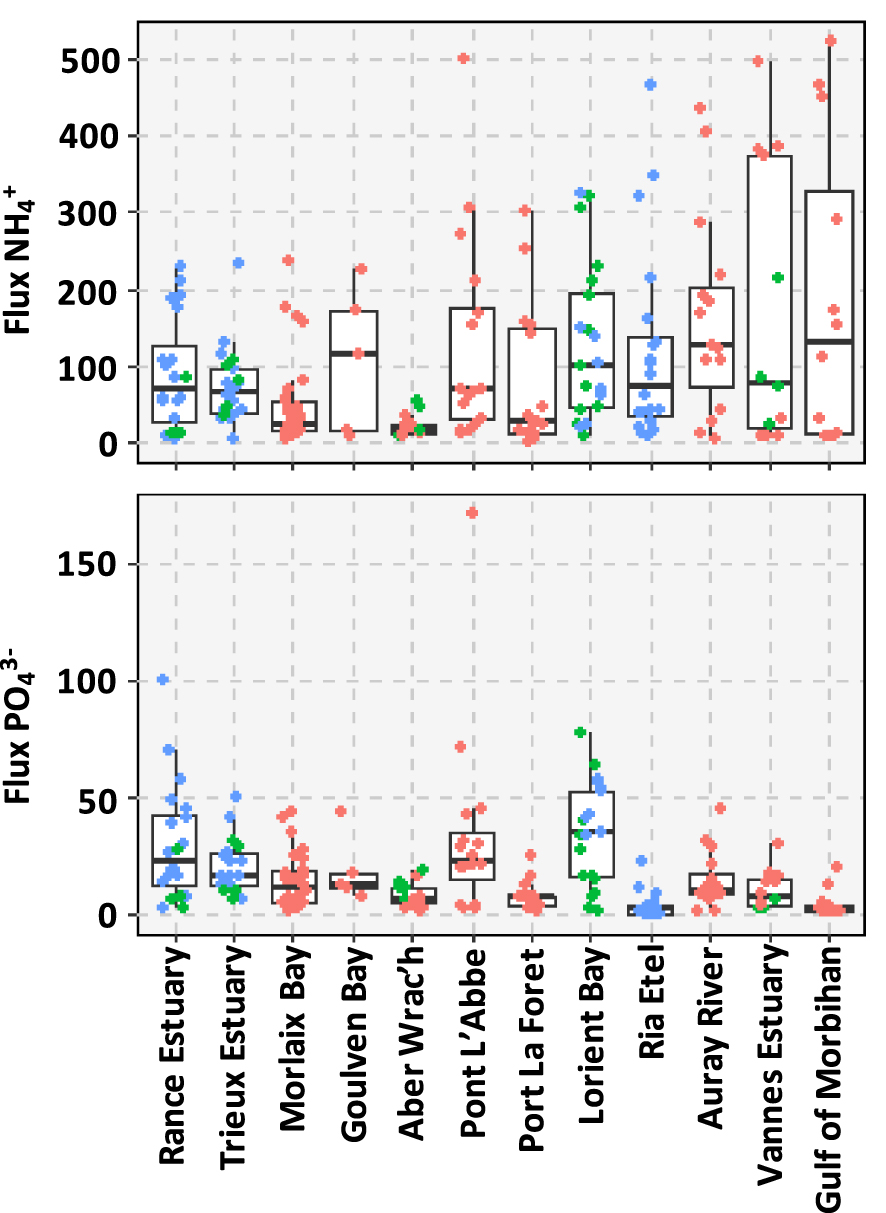
3.2. SOM characterization via isotopic and lipid analysis
3.2.1. Isotopic compositions
The δ13C values varied from −24.3 to −16.2‰, with the highest values measured in the Gulf of Morbihan (mean value = −17.0 ± 0.6‰, sites #43, #44 and #45). Lower values of δ13C (<−22‰) corresponded to sediments collected in the upstream sites of Lorient Bay (sites #13 and #14, mean values = −23.0 ± 0.4‰ and −23.4 ± 1.7‰), the Trieux Estuary (sites #1 and #2, mean values = −22.9 ± 0.3‰ and −23.6 ± 0.5‰), and Port la Forêt (site #31, mean value = 22.6 ± 0.5‰) (Figure 3). The δ15N values varied from 5.8 to 10.5‰. Highest values of δ15N were measured in the Vannes Estuary (site #41, mean value = 9.5 ± 0.7‰), as well as in the Rance Estuary (mean value = 8.4 ± 0.4‰). The lowest values of δ15N were measured in the bay of Aber Wrac’h (site #22, mean value = 6.1 ± 0.3‰). In general, the sediments from middle estuaries were characterized by the highest values of δ15N and the lowest values of δ13C and the opposite was observed for the sediments sampled in the bays (Figure 3).
Ranges of variation of the isotopic ratios δ13C and δ15N as a function of the type of environment.
3.2.2. Distribution and sources of lipids
Considering all the samples, the relative proportion of the five investigated chemical classes is dominated by sterols and stanols (Figure 4). They represent 30 ± 12% (mean ± sd) of the investigated compounds. Fatty acids (FA) and aliphatic hydrocarbons (especially n-alkanes) represented similar proportions of the investigated compounds followed by fatty alcohols. Aromatic hydrocarbons occurred in low proportions in these sediments, representing 2 ± 4%of the investigated compounds.
Ranges of variation of the proportion of the investigated chemical classes among identified compounds.
The distribution of the 17 sterol and stanol compounds were dominated by cholesterol (31 ± 9% of sterol and stanol proportions) and sitosterol (20 ± 6%). Source specific sterols and stanols represented 12 ± 2%, 9 ± 3%, 6 ± 2% and 4 ± 3% for terrestrial plants, phytoplankton [Volkman 1986; Cook et al. 2004], fecal matter [Leeming et al. 1996] and green macroalgae [Iatrides et al. 1983], respectively. This chemical class was composed of 70 ± 5% of ubiquist compounds. The spatial variability of the distribution of the 4 fecal stanols (coprostanol, epicoprostanol, 24-ethylcoprostanol and 24-ethylepicoprostanol) was investigated by a statistical treatment modified from Derrien et al. [2011], Derrien et al. [2012] and Jardé et al. [2018]. This statistical treatment allows the determination of the proportion of the three main fecal matter sources in Brittany (pig slurry, cow manure and waste water treatment plant effluents) into the fecal stanol distribution [Jardé et al. 2018] (Figure S1). The distribution of fecal stanols in the samples resulted mainly from cow manure (68 ± 14%) and pig slurry (11 ± 15%) exports and inputs from waste water treatment plant (WWTP) effluent or non-connected installations (21 ± 8%).
The second most important chemical class in terms of proportion are fatty acid compounds. Fatty acids (FAc) represented 25 ± 11% among the investigated compounds (Figure 4). Their distribution was dominated by nC16:0 that represented 24 ± 4% of FAc. Due to their occurrence in both bacteria and algae [Cranwell et al. 1987; Meziane and Tsuchiya 2000], low molecular weight (LMW) FAc from nC10:0 to nC19:0 were classified as ubiquist, with the exception of iso and anteiso C15:0 and C17:0 that are specific of bacteria. Ubiquist and bacterial FAc represented 66 ± 12% and 5 ± 2% of FAc, respectively. The apparent low proportion of bacterial FAc is due to the fact that a large portion of the LMW FAc was classified as ubiquist. High molecular weight (HMW) FAc from nC20:0 to nC30:0, ω-hydroxy FAc and α,ω diacids originated from terrestrial plants [Eglinton and Hamilton 1967], representing 29 ± 8% of the FAc.
Fatty alcohols (FAl) represented 15 ± 7% of the investigated compounds (Figure 4). Their distribution was dominated by nC24, nC26 and nC28 that represented 15 ± 5%, 26 ± 6% and 16 ± 5% of FAl, respectively. HMW FAl from nC20 to nC30 with a predominance of molecules with an even number of carbon are characteristic of terrestrial plants [Cranwell et al. 1987], representing 86 ± 9% of FAl. The remaining (FAl from nC11 to nC19) were classified as ubiquist due to their occurrence in both bacteria and algae [Cranwell 1974].
The chemical class of aliphatic hydrocarbons represented 26 ± 18% of the investigated compounds and was dominated by n-alkanes (94 ± 5%) (Figure 4). This chemical class exhibits the most variable distribution as highlighted by the mean relative standard deviation that is significantly higher for n-alkanes than for the other chemical classes (Wilcoxon test, p < 0.001). The main compounds of this distribution were nC13 (16 ± 14%) and nC29 (12 ± 6%). The carbon preference index (CPI) ranged from 1.7 to 8.6 with a mean value of 5.0 ± 1.4 (Table 2; Figure 5a). This range highlights that the proportion of crude oil and/or petroleum by-products in the aliphatic fingerprint changed from a low proportion for CPI > 5 to a high proportion for CPI close to 1 [Bray and Evans 1961]. The terrestrial to aquatic ratio (TAR) ranged from 0.9 to 39 with a mean value at 7.2 ± 5.4 (Figure 5b). Only two samples (#44 and #45 in the Gulf of Morbihan) exhibit TAR < 1characteristic of n-alkanes coming mainly from marine sources [Bourbonniere and Meyers 1996]. Out of the 200 samples, 114 have TAR > 5characteristic of n-alkanes originating mainly from terrestrial sources. TAR values from 1 to 5 were deduced for 83 samples, indicating a combination of marine and terrestrial sources. Such variabilities indicate a combination of several sources of OM for this chemical class as highlighted by the different types of chromatograms (Figure 6). The first source (Figure 6a) was characterized by low CPI and the occurrence of a large hump (unresolved complex mixture, UCM) on the chromatogram. This source was also characterized by higher proportion of tricyclic and pentacyclic triterpanes with values of the 22S/(22S + 22R) homohopane that ranged from 0.41 and 0.62 with an average value at 0.53 ± 0.03. This highlights the input of crude oil and/or heavy petroleum by-products such as road asphalt or lubricant oils [Peters and Moldovan 1993]. The second source (Figure 6b) was characterized by a monomodal distribution of LMW n-alkanes from nC11 to nC15 with nC13 as the maximum. This distribution is very similar to the fingerprint of the diesel described by Woolfenden et al. [2011]. The third source (Figure 6c) was characterized by the predominance of HMW n-alkanes (>nC20) with a large odd-over-even predominance resulting in CPI > 5 characteristic of the input of terrestrial plants for n-alkanes from nC25 to nC35 and of emergent aquatic plants from nC21 to nC25. The Paq ratio (Figure 5c) can be used as a balance between these two natural sources [Ficken et al. 2000]. For 109 samples, the proportion of HMW n-alkanes was higher than 50% of n-alkanes and the CPI was higher than 3, indicating that the distribution of n-alkanes was dominated by natural inputs. For these samples, Paq ranged from 0.13 to 0.39 (average value of 0.26 ± 0.06). For Paq < 0.25 (43 samples), the HMW n-alkanes were inherited from only terrestrial plants. The remaining samples (66 samples) are characterized by a combination of terrestrial and emergent aquatic plants (0.25 < Paq < 0.4), which proportions have been determined using an end member mixing approach with 0.25 for terrestrial plants and 0.4 for emergent aquatic plants. The proportion of HMW n-alkanes coming from terrestrial plants in these 66 samples was 65 ± 23% (mean ± SD).
Ranges of variation of ratios calculated on the distribution of n-alkanes. The formulas and diagnostic values are given in Table 2.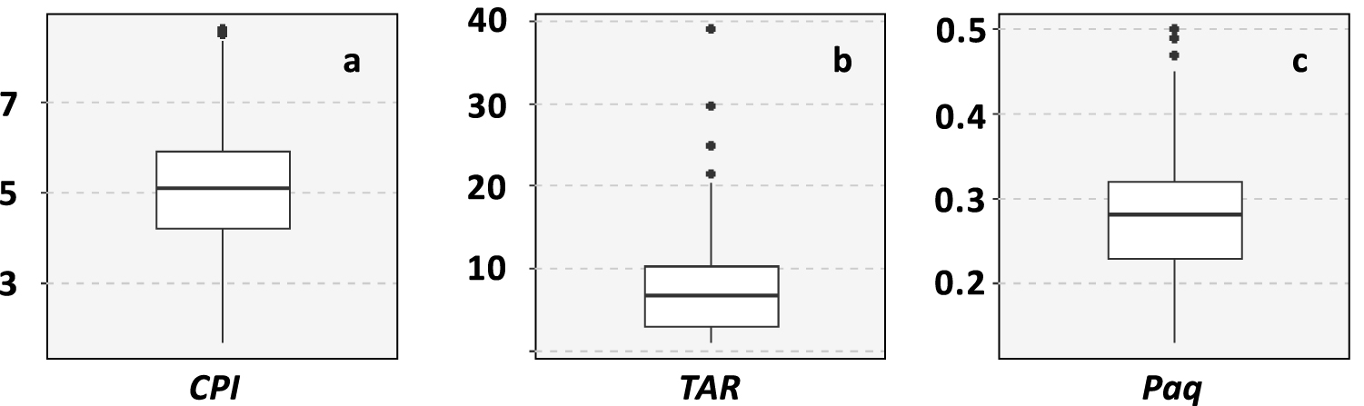
Typical chromatograms of aliphatic fractions from mudflats of Brittany: (a) crude oil dominated chromatogram from Morlaix Bay, site #18; (b) diesel dominated chromatogram from Vannes Estuary, site #40; (c) terrestrial plants dominated chromatogram from Trieux Estuary site #4. Pie charts represent the proportion of molecular markers from terrestrial plants (dark green), algae (light green), microalgae and bacteria (gold), diesel (light grey) and crude oil or heavy refined petroleum by-product (dark grey) in the aliphatic fraction.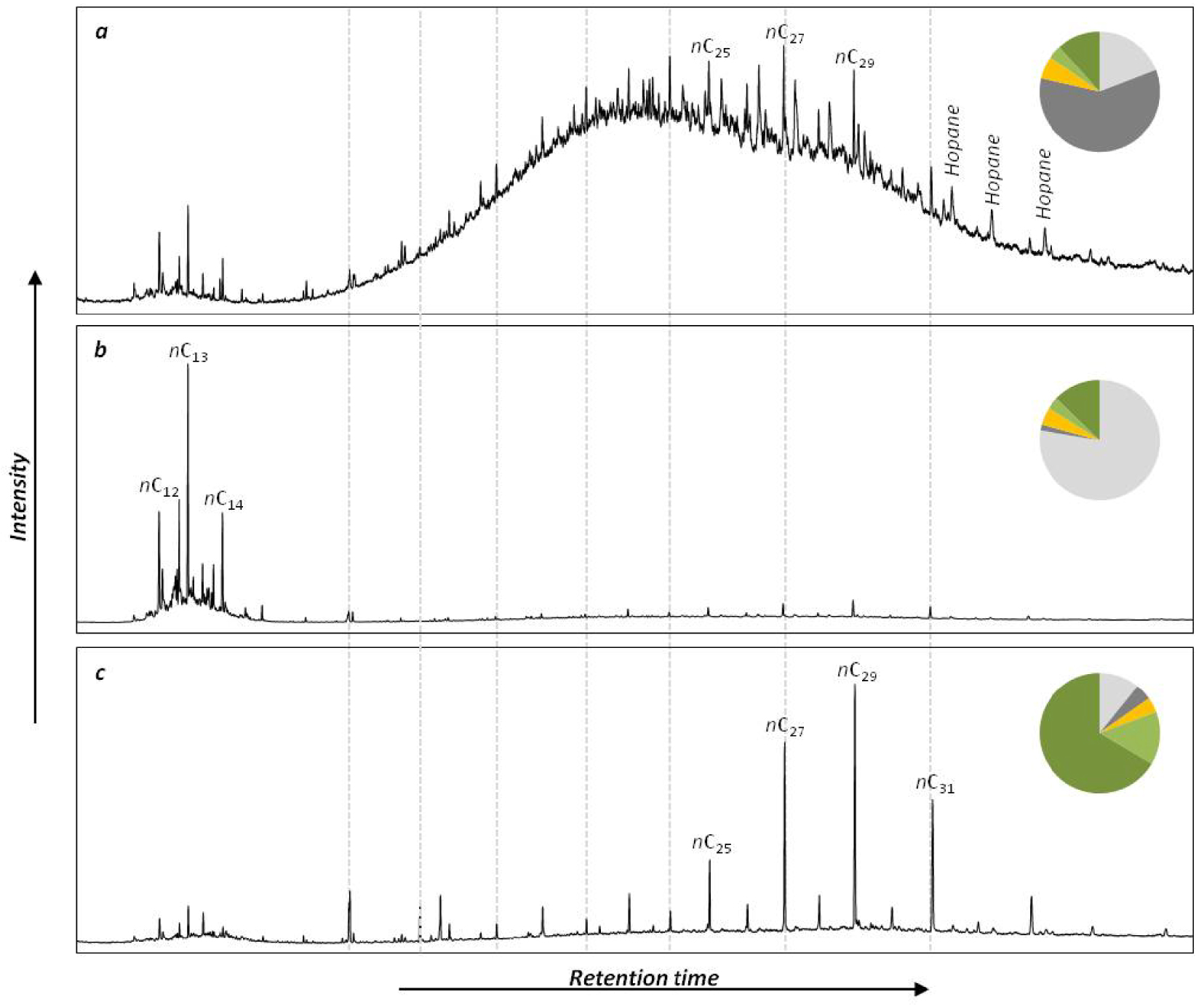
Aromatic hydrocarbons including polycyclic aromatic hydrocarbons (PAHs) represented 2 ± 4% (mean ± sd) of the investigated compounds. This proportion ranged from 0.1 to 47% but is below 5% for the majority (90%) of the samples. Two sites are characterized by high proportion of aromatic hydrocarbons, one in Ria d’Etel (22 ± 18%, site #5) and the other in Auray River (10 ± 5%, site #37). Among this chemical class, the 16 PAHs listed by the US Environmental Protection Agency (EPA) are often quantified in sediments as a measure of the anthropogenic pressure (Figure S2). Their sum was 425 ± 655 ng/g and ranged from 21 to 7489 ng/g of dry sediment. The distribution of PAHs depends on the sources of burned OM and can be used for their identification. The predominance of non methylated PAHs that represented 78 ± 4% (mean ± sd) of PAHs highlighted that they were mainly pyrogenic [Yunker et al. 2002]. Isomeric ratios calculated on PAH allow determining the main pyrogenic source (Table 2; Figure S3). The R4 ratio indicates a combination of pyrogenic OM coming from the combustion of petroleum and modern OM [Yunker et al. 2002]. The R3 ratio indicates a low contribution of wood burning [Yan et al. 2005], while the R1 and R5 ratios indicate emissions from road traffic as the main contributors of this pyrogenic OM [Katsoyiannis et al. 2007; Yunker et al. 2002]. Moreover the R2 ratio highlights that these particles have been aged by photolysis [Oliveira et al. 2011].
3.3. Variance partitioning and canonical redundancy analysis
Significant variables from the various datasets were selected to determine the relationship between biodegradability and OM sources while taking the sediment properties into account. The grain-size distribution, the porosity, the elemental composition of bulk OM and benthic nutrient fluxes were taken from Louis et al. [2021]. Benthic and fluxes are shown in Figure 6. In the “SOM origin” data matrix, the selected variables were δ13C values, δ15N values, and six lipid marker groups: “Fecal”, “Petroleum products”, “Microalgae”, “Plants 3”, “Plants 4” and “Bacteria 1” (see Table 1 for the composition of these groups). Regarding the “physico-chemical composition” data matrix, the selected variables were the Fe-P, Org-P and the porosity. With these selected variables in both data matrices, the variance partitioning of the and fluxes was carried out and the results are presented in Figure 7. The selected “SOM origin” and “physico-chemical composition” parameters explained 30 and 34% of the variance of the and fluxes respectively. The variables related to “SOM origin” significantly explained 16% of the variance of the fluxes (F = 5.3, p = 0.001) and 16% of the variance of fluxes (F = 5.8, p = 0.001), compared to 6 and 3% with the “physico-chemical composition” variables. The “SOM origin” and “physico-chemical composition” variables shared between 8 and 15% of the variance partitioning of the and fluxes, respectively.
Variation partitioning of the and fluxes. “SOM origin” corresponds to δ13C values, δ15N values and the proportions of the lipid marker groups. “Physico-chemical composition” corresponds to the selected parameters related to the composition (Fe-P, Org-P) and physical properties (porosity) of the sediment.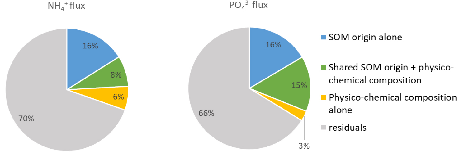
In order to relate the benthic nutrient fluxes with the selected variables from the SOM origin, the isotopic composition and the physical and chemical properties, a canonical redundancy analysis (RDA) was performed (Figure 8). A total of 32.1% of the variance in combined benthic fluxes of and was explained by the eleven selected parameters (permutation test: F = 7.99; p = 0.001). The first canonical axis (F = 59.55; p = 0.001) represents 64.6% of the constrained variance (20.7% of the total variance) of benthic fluxes data, and is explained by Fe-P (r = 0.67; p = 0.043), porosity (r = 0.65; p = 0.014), P-Org (r = 0.62; p = 0.021), Fecal markers (r = 0.61; p = 0.001), δ15 N values (r = 0.42; p = 0.02) and Microalgal markers (r = 0.38; p = 0.001). The second canonical axis (F = 32.63; p = 0.001) represents 35.4% of the constrained variance (11.4% of total) of benthic fluxes data, and is mainly explained by the δ13C values (r = −0.76; p = 0.002), followed by Petroleum products markers (r = −0.40; p = 0.001). The fluxes were positively correlated with the first axis (r = 0.64) and negatively with the second axis (r = −0.77). The fluxes were positively correlated with the first axis (r = 0.77) and the second axis (r = 0.64). Finally, the RDA showed a positive association between the fluxes and the Org-P and Fe-P contents as well as the proportions of fecal markers. For the fluxes, a positive association was observed with δ13C and δ15N values, the porosity and the proportions of microalgal and petroleum product markers.
Correlation circles of the Canonical Redundancy Analysis (RDA) showing the correlations between (a) the explanatory variables, related to the SOM origin (in red), isotopic composition (in blue) and physico-chemical properties (in black) of the sediment, and (b) the response variables ( and fluxes).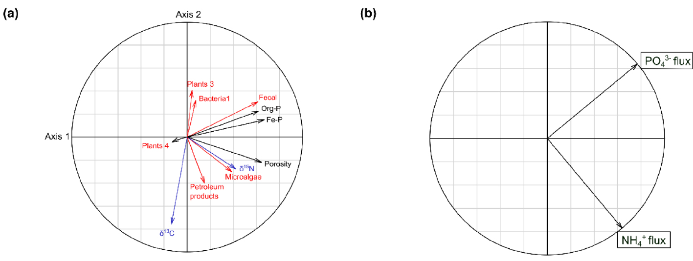
4. Discussion
4.1. What is the spatial variability in the origin of SOM?
In the investigated mudflats, the SOM originated from several natural and anthropogenic sources.
The natural OM sources included terrestrial plants, bacteria, freshwater algae, marine phytoplankton, microphytobenthos, as well as Ulva sp., a green macroalgae highly present along the coast of Brittany. From 2008 to 2020, the average surface of stranded Ulva on mudflats was 1284 ha (Environmental Observatory of Brittany). The lipids present in the mudflats of Brittany were mainly of natural origin. Their proportion, including ubiquist compounds from natural sources such as cholesterol and LMW FAc, ranged from 24% (Auray River, site #39) to 97% (Ria Etel, site #6) of the analyzed compounds with a mean value of 81 ± 15% (mean ± SD) (%Nat—Figure 9). The isotopic data and the distribution of n-alkanes indicated spatial variations of the contribution of these primary producers to the SOM. From middle estuaries to bays, δ15N values and TAR decreased while δ13C values and Paq increased with significant differences between bays, lower estuaries and middle estuaries, with the exception of TAR for which the only significant difference was between bays and middle estuaries.
Ranges of variation of ratios calculated on the distribution of lipids. %Nat is the proportion of natural markers among all identified compounds, including ubiquist compounds. %Terr is the proportion of terrigenous markers among all identified compounds, including ubiquist compounds. %Diesel is the proportion of diesel markers among petrogenic markers.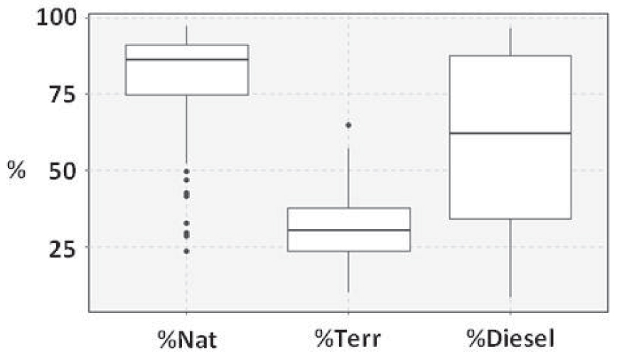
Based on the isotopic shift between C3 terrestrial plants [δ13C = −28.7 ± 0.5‰ Davoult et al. 2017; Meyers 1994] and marine organisms [phytoplankton δ13C = −21.3 ± 1.2‰; Liénart et al. 2017 and Ulva sp. δ13C = −15.8 ± 4.4‰; Berto et al. 2013; Dubois et al. 2012; Riera et al. 1996], the increase in δ13C values along the estuaries was associated to an increasing proportion of marine OM. This was reinforced by the correlations between δ13C values and the proportion of terrestrial markers among identified compounds (%Terr—Figure 9) (r = −0.33; p < 0.0001), the Paq (r = 0.53; p < 0.0001) and TAR (r = −0.39; p < 0.0001) ratios quantifying the terrestrial versus aquatic or marine origin of n-alkanes. From middle estuaries to bays the proportion of aquatic, calculated using the Paq ratio, and marine, calculated using the TAR ratio, n-alkanes increased, indicating an increase in the proportion of SOM inherited from marine organisms, which was recorded by the rise in δ13C values. Such a trend was in accordance with observations in other estuaries around the world [Ankit et al. 2017; Chevalier et al. 2015; Gireeshkumar et al. 2015; Lopes dos Santos and Vane 2020].
Microbial transformations of nitrogen induce changes in δ15N values due to the enzymatic preference for the lighter 14N. Therefore, the anthropogenic inputs from WWTP and agriculture, subject to microbial activity, generally show an increase in adjacent sedimentary δ15N values [Finlay and Kendall 2007; Rumolo et al. 2011; Savage 2005]. The occurrence of WWTP, individual septic systems and the elevated agricultural density (80% of the area) are both potential sources in the current study. When considering all the samples, δ15N values negatively correlated with the Paq n-alkane ratio (r = −0.34, p < 0.0001). High δ15N values were associated with high proportion of terrigenous n-alkanes. Since Brittany is a highly agricultural area, we assume that terrigenous n-alkanes were indicators of soil erosion and thus of agricultural inputs. δ15N values were also positively correlated with the proportion of human fecal stanols among analyzed compounds (r = 0.15, p = 0.035). Consequently the δ15N values indicated that mudflats of Brittany would be influenced by both waste water management and agricultural practices.
Overall, the correlations between isotopic and lipid data were relatively weak, which could be due to the fact that isotopic data result from the combination of all the sources of OM (natural and anthropogenic ones). Lipid analysis highlighted four sources of anthropogenic OM. Two are characteristic of petroleum products: diesel and potentially degraded crude oil. Both of these contaminations occurred in all mudflat sediments with variable proportions as indicated by the ratio diesel/petrogenic (%Diesel—Figure 9). The petrogenic contamination was mainly due to crude oil in Northern mudflats, while diesel dominated in Southern mudflats, with the exception of the Rance Estuary in the north, the Lorient Bay and the Ria d’Etel in the south. Compared to Northern mudflats, the Rance Estuary sediments were enriched with diesel (p < 0.01), which could be due to the low hydrodynamics induced by the tidal power plant that closes this estuary since the 60’s [Rtimi et al. 2021]. Compared to Southern mudflats, the concentration of diesel markers were lower in the Lorient Bay (p < 0.001) and the Ria d’Etel (p < 0.001). Since the land use is very similar in upstream areas along the southern coast, these differences could be due to a combination of geomorphological and hydrological conditions that could impact the sedimentation of diesel droplets [Gearing et al. 1980].
The third source of anthropogenic OM was pyrogenic and was characterized by the occurrence and the distribution of PAHs [Yunker et al. 2002]. Its occurrence in mudflat sediments, quantified by the sum of the concentration of the 16 PAHs listed by the US-Environmental Protection Agency (US-EPA) was in the same range but slightly higher than in the European Northern Sea and the Baltic Sea [Wang et al. 2020]. The background contamination in sediments of the eastern North Atlantic has been determined by the OSPAR commission, a cooperation between 15 governments and the European Union to protect the marine environment of the North-East Atlantic (OSPAR, 2017). Among the present samples, 24% of the mudflat sediments presented higher contamination levels than this background. Most of these were from the Ria d’Etel (25% of the contaminated sediments), Auray River (23%) and Lorient Bay (21%). Isomeric ratios calculated on PAH allowed identifying particles coming from the emissions from road traffic and aged by photolysis as the main pyrogenic source (Figure S3). This was in agreement with one of the main source of PAHs identified in Northern and Baltic seas [Wang et al. 2020].
Finally, the anthropogenic OM from fecal contaminations was highlighted by the occurrence and the distribution of fecal stanols. The sum of their concentrations ranged from 4 to 1934 ng/g of dry sediment (276 ± 261 ng/g; mean ± sd). This was 10 times lower than in the Tay Estuary (Scotland) before the building of a WWTP [Reeves and Patton 2005] and 5 times lower than the mean concentrations in Jinhae Bay (South Korea) [Choi et al. 2002]. Only 4 samples of the study exhibited a coprostanol concentration higher than 500 ng/g, which has been suggested as the threshold to indicate a significant fecal contamination [Leeming and Nichols 1996]. Based on this, fecal contamination was small in mudflat sediments along the Brittany coastline. This fecal contamination resulted mainly from cow manure (68 ± 14%) and pig slurry (11 ± 15%) exports and inputs from WWTP effluent or non-connected installations (21 ± 8%), which was in accordance to the combination of sources of fecal contamination that has been determined in rivers of Brittany [Jardé et al. 2018].
4.2. How the origin of SOM impacts benthic nutrient fluxes?
The origin of SOM has often been suggested as a driver of SOM biodegradation and benthic nutrient fluxes [LaRowe et al. 2020]. This large dataset allowed for the first time to significantly quantify this relationship for and fluxes produced by mudflats in tidal environments. The benthic and fluxes, measured from the sediment core incubations, were significantly correlated (p < 0.005) to the SOM origin. The percentage of variance for the and fluxes explained only by the “SOM origin” variables was 16%, compared to 6% (for fluxes) and 3% (for fluxes) for the “physico-chemical composition” variables. By combining all variables, the explained percentage of variance for the and fluxes reached 30 and 34% respectively. The origin of SOM was thus a significant driver of benthic nutrient fluxes. The RDA highlighted that the and fluxes were not correlated to the same variables.
The flux was positively related to the isotopic signature of the bulk sediment OM (δ15N and δ13C values), the porosity and the proportions of microalgal and diesel markers. In geographically closed areas, low hydrodynamic conditions improve the sedimentation of (i) fine particles, increasing the porosity of sediments [Meade 1966] and (ii) diesel droplets lighter than seawater through flocculation. In such low hydrodynamic conditions, the development of microalgae promoted by anthropogenic N coming from watersheds and their sedimentation must have brought to the sediment 13C-enriched [Cook et al. 2004; Li et al. 2016; Ogrinc et al. 2005] and 15N-enriched [Savage 2005; Finlay and Kendall 2007; Rumolo et al. 2011] marine OM, increasing the proportion of microalgal markers in the lipidic fraction of SOM. Phytoplanktonic blooms are known to enrich sediments in nitrogen and labile SOM [Franzo et al. 2019]. These inputs have promoted a quick response of the bacterial reactivity in the sediment [Hardison et al. 2013; Pruski et al. 2019], which has induced seasonal variability in benthic nitrogen fluxes [Grenz et al. 2000]. The present results showed that phytoplanktonic blooms could also be responsible for spatial variability in benthic nitrogen fluxes from mudflat sediments. The flux was thus partially controlled by the origin of SOM that might have been driven by the geomorphology. Under low hydrodynamic conditions, an algal bloom might have been stimulated, especially if the coastal system was impacted by nitrogen loading from the watershed, and thus become an OM source for the coastal sediment.
The geographical configuration of the Gulf of Morbihan which opens onto the Atlantic Ocean through a narrow passage 850 m wide and covering an area of 115 km2 illustrated perfectly these relationships between geomorphology, origin of SOM and benthic flux. This area combined the samples from the Auray River, Vannes and the southern internal coast of the Gulf (Figure 1). In this area, the porosity was significantly higher (p < 0.0001) than in other mudflats, which indicated an area with low hydrodynamic conditions. These conditions have improved the assimilation of dissolved anthropogenic nitrogen by microalgae and their sedimentation. Higher sedimentation rates were emphasized by significantly higher proportions of diesel markers in this area (p < 0.0001). As a consequence, SOM was enriched in OM from microalgae as indicated by significantly higher δ15N (p < 0.01), δ13C (p < 0.0001) and microalgal markers (p < 0.001), which induced a mean flux that was two times higher than in the other mudflats of Brittany (p = 0.001).
This link between topography, algal bloom, sedimentation and enrichment in sedimentary heavy nitrogen seems in accordance with the main mode of export of nitrogen from agricultural watersheds that is mainly under dissolved form [Mulholland et al. 2008]. Before storage in mudflat sediments, N must be fixed by aquatic primary producers. In 2021, the mean Q90 (the value below which at least 90% of the data fall) nitrate concentration at the regional scale was 41 ± 25 mg/L (data from the Environment Observatory in Brittany). Consequently, reducing benthic N fluxes from mudflat sediments will require a decrease in the dissolved N fluxes from agricultural catchments and then a decrease in the amount of N fertilizers used by the chemical conventional agriculture to avoid N-surplus [Leip et al. 2011].
The flux was positively related to the proportion of fecal markers, as well as the Org-P and Fe-P. Fecal markers occurring in the investigated mudflats originated mainly from the erosion of agricultural soils amended with bovine manure and pig slurry (79 ± 29%) and from WWTP and individual septic systems (21 ± 8%). This finding seems to be in accordance with the increase in fluxes via a larger dissolution rate of Fe-P due to reductive conditions in sediments impacted by urban and agricultural activities in the Bay of Brest in Brittany [Khalil et al. 2018]. Biogeochemical modelling used to investigate the mechanisms behind these relationships has highlighted the role of the input of labile OM from urban and agricultural activities. This would have led to high mineralization rates and in the increase in fluxes through both mineralization and subsequent reductive Fe-P dissolution [Ait Ballagh et al. 2020].
Org-P and Fe-P in sediments may come from direct sedimentation of particulate Org-P and Fe-P exported by watersheds or from sedimentation of marine primary producers that would have assimilated dissolved P [Watson et al. 2018]. In rivers of Brittany, over the period 2007 to 2011, the mean fluxes of particulate P has been 1.7 times higher than the mean fluxes of dissolved P [Bol et al. 2018]. The correlations between sedimentary P stocks and δ13C (Org-P: r = −0.21, p < 0.01; Fe-P: r = −0.32, p < 0.001), Paq (Org-P: r = −0.27, p < 0.001; Fe-P: r = −0.30, p < 0.001) and the concentration of fecal markers (Org-P: r = 0.40, p < 0.001; Fe-P: r = 0.37, p < 0.001) seems to indicate that sedimentary P stocks were mainly associated with terrestrial OM. This could highlight particulate P as the main source of sedimentary P through soil erosion. Moreover the median benthic fluxes were positively correlated to the watershed area (r = 0.8, p < 0.001). Intensive agricultural activities cover 60% of the area in Brittany and result in one of the world’s largest P surpluses [MacDonald et al. 2011], which may affect the sediment composition through agricultural soil erosion, which can be considered as a transport vector of fecal matter and particulate phosphorus. Therefore, benthic fluxes seem to be driven by the surface area of the watersheds and the land use in the catchment. Consequently, agricultural practices allowing a decrease in P surplus and soil erosion should induce a decrease in sedimentary P stocks and then a decrease in benthic fluxes.
4.3. A large proportion of the variance of benthic nutrient fluxes remained unexplained
In the present study, we focused on the link between the benthic nutrient fluxes and the sediment composition, while comparing the significant effect of SOM origin versus quantity. Nevertheless, a large part of the variance in the benthic and fluxes on the regional scale remained unexplained (70 and 66%, respectively) (Figure 7). Microbial abundance and diversity were not assessed in the current study, and abundance and/or diversity may play an additional role in nutrient cycling. As shown by Abell et al. [2013], the composition of the bacterial community has been related to the nature of the OM in estuarine systems, and their combination may lead to a shift in the benthic nutrient fluxes. In addition, bioturbation, mediated by macrofauna activities, was likely present in the sediment core incubations and possibly involved in the spatial variability of the and fluxes. Bioturbation includes particle reworking and burrow ventilation, promoting exchanges of solute between the porewater and the overlying water and stimulating microbial activities [Graf and Rosenberg 1997]. The review and experimental studies of Karlson et al. [2007] and Renz and Forster [2014] have highlighted the stimulation of the and effluxes by benthic macrofauna, with a magnitude that varied according to the density, burrowing depth and ventilation of polychaetes and bivalves. Bioturbation promotes effluxes through the mineralization of SOM via an additional supply of electron acceptors (e.g. oxygen, nitrate), the remobilization of burial OM, and excretion from macrofauna [Welsh 2003, and references therein]). The release of in the presence of macrofauna also depends on the sediment redox status and components (e.g iron oxides). In fact, bioturbation increases P-Org mineralization and then regenerated can be either released by porewater flushing or adsorbed into iron oxides under oxic conditions. Therefore, Nizzoli et al. [2007] observed that the bioturbation by polychaete Nereis spp. had site specific effects on the flux, with sediment acting either as a sink or a source of .
5. Conclusion
To the best of our knowledge, this is the first study that describes the variability in the SOM origin through a broad sampling campaign of marine mudflats at the regional scale (Brittany), relating SOM origin to benthic nutrient fluxes. The combination of isotopic and lipid data emphasized the SOM in Brittany intertidal mudflats as a mixture of natural (marine and continental) and anthropogenic OM. Its composition varied according to the anthropogenic pressures of watersheds as well as the hydrodynamic conditions. Benthic nutrient fluxes were significantly driven by the origin of SOM that explained 24% and 31% of the variance of and fluxes, respectively. Benthic nutrient fluxes were linked to terrestrial export of N and P but were not correlated to the same parameters. The fluxes were driven by the uptake by phytoplankton of dissolved anthropogenic N exported from agricultural catchments. Their sedimentation was favoured by low hydrodynamic conditions, enriching the sediments with labile OM. The fluxes were driven by the sedimentation of particulate P exported through agricultural soil erosion.
A significant fraction of the spatial variability in the benthic nutrient fluxes remains unexplained by the investigated sedimentary characteristics. The spatial variability of benthic macrofauna and microbial biomass might play a role in this unexplained variance and should be considered in future investigations.
Conflicts of interest
The authors declare that they have no conflict of interest.
Acknowledgments
This work was funded by Loire-Bretagne Water Agency and the Regional Council of Brittany (France). It was carried out as a part of the IMPRO research project. The authors would like to thank Josette Launay (CRESEB) for the project coordination. The authors would also like to thank P. Petitjean, C. Petton, G. Bouger, O. Jambon and C. Roose-Amsaleg for their assistance in the field. The CEVA, the Syndicat Mixte EPTB Rance-Fremur, the Pays de Guingamp, the Syndicat Mixte des Bassins du Haut-Léon, the Syndicat des Eaux du Bas-Léon, Lorient-Agglomération, the Syndicat Mixte du SAGE Ouest-Cornouaille (OUESCO), Concarneau-Cornouaille-Agglomération, the Syndicat Mixte de la Ria d’Etel (SMRE) and the Syndicat Mixte du Loc’h et du Sal (SMLS) are acknowledged for their help preparing the field campaign. The authors would also like to thank O. Lebeau (Plateforme Isotopes Stables, IUEM) for the elemental and isotopic analyses, and Marie-Claire Perello (EPOC, University of Bordeaux) for the particle-size analyses. S. Mullin is acknowledged for carefully checking the English content. Two anonymous reviewers are acknowledged for improving the quality of this manuscript.
Supplementary data
Supporting information for this article is available on the journal’s website under https://doi.org/10.5802/crgeos.228 or from the author.