Version française abrégée
Dans l’analyse du changement climatique simulé par les modèles couplés, il semble de plus en plus important de prendre en compte les dépendances d’échelle et les statistiques d’ordre plus élevé. Le formalisme multifractal, développé pour l’étude de la turbulence, est un outil théorique approprié pour caractériser de façon parcimonieuse les statistiques de tous ordres, et sur une grande gamme d’échelles, qui a été appliqué avec succès à l’analyse de l’invariance d’échelle des champs de précipitation. Il est appliqué ici à l’analyse des séries quotidiennes de précipitations sur la France, calculées par le modèle de climat CNRM-CM3 de Météo France dans une simulation climatique couplée d’évolution du climat futur, réalisée pour le GIEC selon le scénario A2 [25]. La méthodologie est d’abord résumée en rappelant les définitions des deux exposants caractérisant l’invariance d’échelle. Le premier, c(γ) caractérise la loi d’échelle de la probabilité de dépassement d’un seuil, lui-même écrit sous forme de la puissance γ du rapport d’échelle (éq. (1)), γ étant l’ordre de singularité. Le deuxième, K(q), caractérise les moments d’ordre q (éq. (2)). Sous des conditions assez générales, quelques paramètres peuvent suffire à caractériser ces exposants, notamment dans le cadre du modèle multifractal universel, qui est un cas limite pour les cascades multiplicatives [27,29] : le degré ou index α de multifractalité du champ étudié (0 ≤ α ≤ 2 : α = 2 correspond au cas maximal de multifractalité, souvent (improprement) dénommé « log-normal », α = 0 correspond au contraire au cas d’uni/monofractalité), et la codimension de la singularité moyenne C1 qui caractérise l’intermittence (moyenne), c’est-à-dire l’inhomogénéité du champ moyen (C1 = 0 correspond à un champ totalement homogène). Les équations (3) et (4) fournissent les expressions analytiques les reliant à c(γ) et K(q). La technique utilisée pour l’analyse multifractale est celle du moment double trace DTM (de l’anglais double trace moment [13,30]), qui permet de déterminer directement les paramètres α et C1 caractéristiques de la série utilisée. Pour sa mise en œuvre, on introduit un champ des puissances η, normalisées, du champ initial (équation (5)). En utilisant plusieurs valeurs de η, les paramètres α et C1 peuvent être déterminée dans un diagramme log–log, les exposants K(q,η) étant déterminés au préalable sur les parties linéaires (caractérisant la plage de symétrie d’échelle révélée par la série) des courbes obtenues par dégradation de la résolution du champ initial.
Les séries de précipitations ont été simulées par le modèle couplé océan–atmosphère–glace du Centre national de recherche météorologique de Météo France (version CNRM-CM3) sur la période allant de 1860 à 2000, à partir des concentrations observées des gaz à effet de serre, puis sur le xxie siècle, en suivant le scénario A2 du GIEC [25]. Les séries journalières des précipitations sont fournies sur une grille d’une taille de 2,8 × 2,8°, soit des mailles d’environ 200–300 km de côté, pour 12 points de grille sur la France métropolitaine (Fig. 1). Les simulations montrent une décroissance des précipitations moyennes et une augmentation des précipitations maximales qui s’accélère au cours du xxie siècle, particulièrement dans le Sud de la France (Fig. 2).
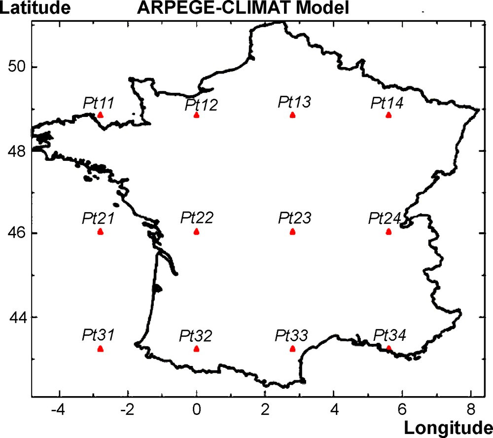
Geographical position of the model grid points Ptij with: i = 1,4 (longitude: from west to east); j = 1,3 (latitude, from north to south).
Position géographique des points de grille du modèle Ptij avec i = 1,4 (longitude : de l’ouest vers l’est) ; j = 1,3 (latitude, du nord vers le sud).
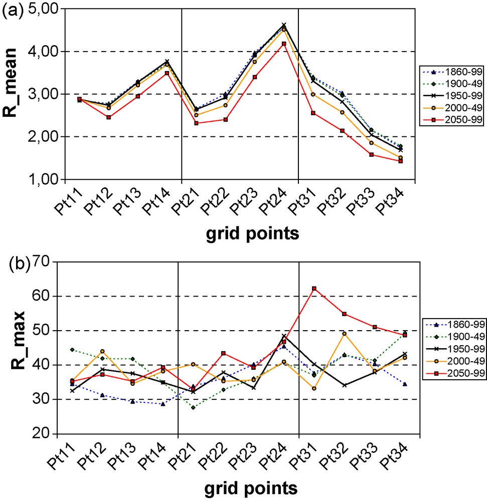
Variation depending on the grid point location of the mean precipitation in mm/day (a) and the maximum daily precipitation (b) over successive time spans. The horizontal axis is indexed by n = j + 4 (i − 1) with respect to the indices in Fig. 1, and the different latitudes (indexed by j) from north to south are separated by vertical lines.
Variation selon l’emplacement des points de grille de la précipitation moyenne en millimètres par jour (a) et du maximum des précipitations quotidiennes (b), simulés par le modèle pour des intervalles de temps successifs. L’axe horizontal est indicé par n = j + 4 (i − 1) par rapport aux indices de laFig. 1, et les différentes latitudes (indexées par j) du nord au sud sont séparées par des traits verticaux.
L’analyse spectrale des séries (Figs. 3 et 4), puis l’analyse multifractale par la méthode DTM, met en évidence une symétrie d’échelle allant jusqu’à 16 jours (Fig. 5). Seuls les résultats sur 50 ans sont présentés dans cette étude, mais ils ont été confirmés par des analyses similaires sur des séries de 25 et 10 ans. Les paramètres α et C1 présentent une certaine variabilité géographique, mais évoluent de façon monotone au cours de la simulation : augmentation pour l’intermittence C1 et décroissance pour la multifractalité α (Fig. 6). L’évolution de C1 est conforme à l’augmentation des séquences de jours sans précipitation au cours du xxie siècle. L’évolution en sens inverse de C1 et α conduit à une certaine compensation de leurs effets sur l’exposant des moments K(q), mais l’effet de C1 reste prépondérant.
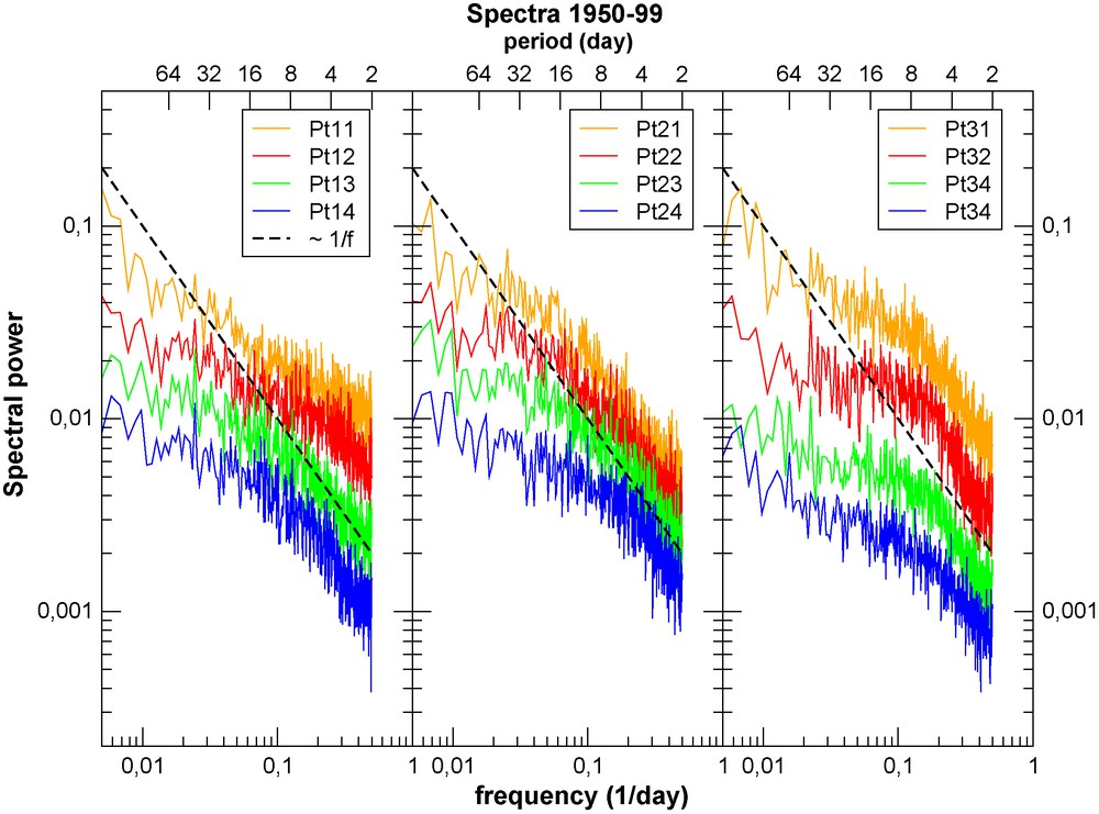
Spectral analysis of the simulated rain field (at the 12 grid points): the power spectra result from the average over a 50-year simulation period (1950–1999) of the spectra computed over consecutive 1024 day durations. The plot is in logarithmic coordinates with frequency f (in day−1) on the lower horizontal axis and period (in days) in the upper horizontal axis. The spectra have been grouped by latitude bands, and offset downward arbitrarily (to separate them) over the longitudes from west to east. Over the frequency range corresponding to 2 to 16 days, they clearly follow a power law (E(f) ≈ f–β) with a spectral slope β < 1, except for point Pt32, where the slope is slightly above 1 and the linear part limited to 8 days (the dashed line corresponds to a slope β = 1). Masquer
Spectral analysis of the simulated rain field (at the 12 grid points): the power spectra result from the average over a 50-year simulation period (1950–1999) of the spectra computed over consecutive 1024 day durations. The plot is in logarithmic coordinates ... Lire la suite
Analyse spectrale des champs de pluie simulés (aux 12 points de grille) : ces spectres de puissance sont une moyenne, sur une période de 50 ans (1950–1999), des spectres calculés sur des durées consécutives de 1024 jours. Le diagramme est en axes logarithmiques avec la fréquence f (en j–1) sur l’axe horizontal inférieur et la période (en j) sur l’axe horizontal supérieur. Les spectres ont été groupés par bandes de latitude, et décalés arbitrairement vers le bas (afin de les distinguer) pour les longitudes allant de l’ouest vers l’est. Sur la gamme de fréquence de 2 à 16 jours, ils suivent visiblement une loi de puissance (E(f) ≈ f–β), avec des pentes spectrales β < 1, excepté pour le point Pt32, où la pente est un peu supérieure à 1 et la partie linéaire limitée à 8 jours (la ligne pointillée correspond à une pente β = 1). Masquer
Analyse spectrale des champs de pluie simulés (aux 12 points de grille) : ces spectres de puissance sont une moyenne, sur une période de 50 ans (1950–1999), des spectres calculés sur des durées consécutives de 1024 jours. Le diagramme est ... Lire la suite
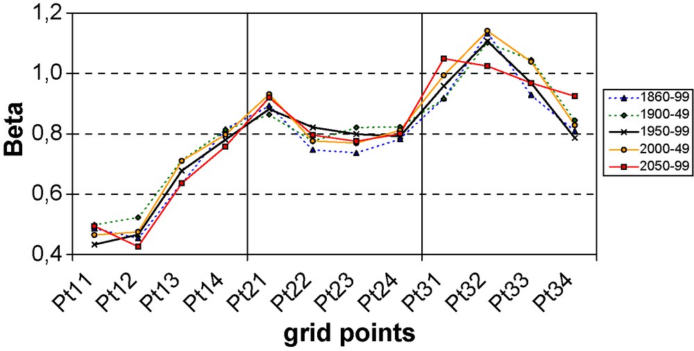
Variation of spectral slope β of the linear part of the spectrum (E(f) ≈ f–β) depending on the grid point location and the time range over which they are estimated (as in Fig. 2)
Variation de la pente spectrale β de la partie linéaire du spectre (E(f) ≈ f–β), selon l’emplacement des points de grille et les intervalles de temps sur lesquels ils sont estimés (comme sur laFig. 2).
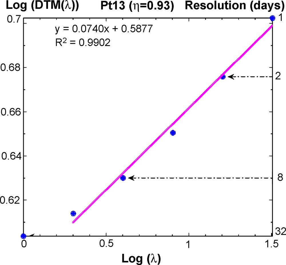
Illustration of the DTM first step (at the grid point Pt13): determination of K(q,η) as the slope of the log–log of the Double Trace Moment (of order q = 1.5 and power η = 0.93) vs. its time resolution λ.
Illustration de la première étape du DTM (au point de grille Pt13) : détermination de K(q,η) en tant que pente sur le tracé en échelle log–log du moment double trace (d’ordre q = 1,5 et de puissance η = 0,93), en fonction de sa résolution temporelle λ.
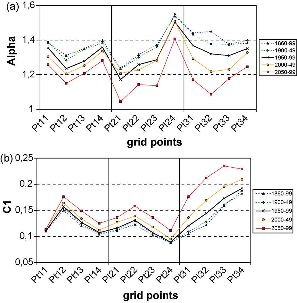
Variation of α (a) and C1 (b) depending on the grid point location and the time range over which they are estimated (as in Fig. 2).
Variation de α (a) et de C1 (b) selon l’emplacement des points de grille et les intervalles de temps sur lesquels ils sont estimés (comme sur laFig. 2).
La notion de singularité maximale presque jamais dépassée γs, définie par la relation (6), permet de caractériser une invariance d’échelle pour les extrêmes (équation (7)). Ce paramètre peut être calculé analytiquement à partir de C1 et α (équation (8)). Au cours des simulations, la singularité maximale tend à augmenter (Fig. 7). Un diagramme de dispersion montre que l’évolution de γs correspond bien à celle de la précipitation maximale (Fig. 8). L’analyse multifractale permet de relier ces changements à une évolution antagoniste entre l’intermittence C1 et la multifractalité α (Fig. 9).
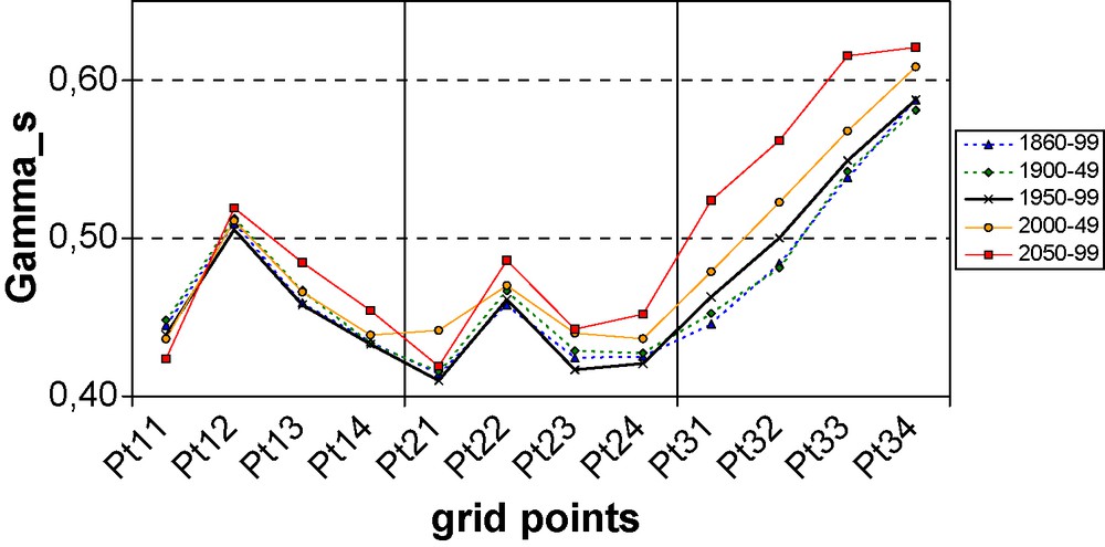
Variations of the maximal probable singularity γs depending on the grid points and the time range over which they are estimated (as in Fig. 2).
Variations de la singularité maximale probable γs, selon l’emplacement des points de grille et les intervalles de temps sur lesquels ils sont estimés (comme sur laFig. 2).
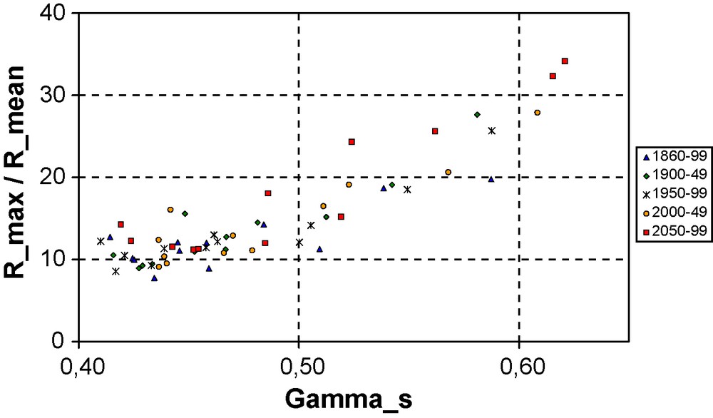
Dispersion diagram showing the ratio of maximum to mean precipitation (Rmax/Rmean) as a function of the maximal probable singularity γs for the different grid points and time intervals.
Diagramme de dispersion montrant le rapport de la précipitation maximale à la précipitation moyenne (Rmax/Rmean), en fonction de la singularité maximale γspour les divers points et les divers intervalles de temps.
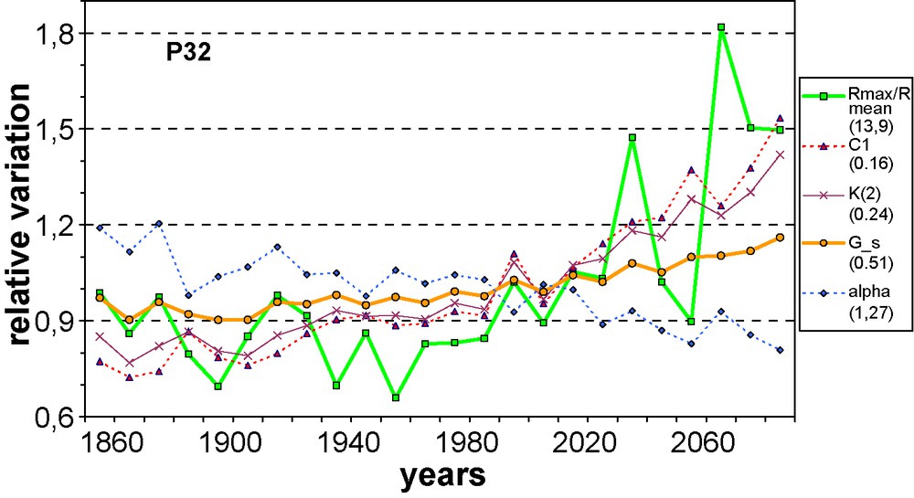
Time series illustrating the relative evolution of parameters at point Pt32 during the period 1860–2099. In order to make their scales comparable, the values of each parameter, computed over successive 10-year time slices, have been normalized by dividing them by their average over the whole period (indicated within parentheses in the legend). The parameters are: α, multifractality index (alpha: lozenges, dashed line); C1, intermittency coefficient (C1: triangles, dashed line); K(q), moment scaling function of order q = 2 (K(2): crosses, thin line); γs, maximum singularity (G_s: circles, thick line); Rmax/Rmean, ratio of the maximum daily rainfall for each 10 years to the mean rainfall (Rmax/Rmean: squares, thick lines). Masquer
Time series illustrating the relative evolution of parameters at point Pt32 during the period 1860–2099. In order to make their scales comparable, the values of each parameter, computed over successive 10-year time slices, have been normalized by dividing them by ... Lire la suite
Séries temporelles illustrant l’évolution relative des paramètres au point Pt32 pendant la période 1860–2099. Pour rendre comparables leurs échelles, les valeurs de chaque paramètre, calculées sur des tranches de 10 ans successives, ont été normalisées en les divisant par leur moyenne sur toute la période (indiquée entre parenthèses sur la légende). Les paramètres sont : α, indice de multifractalité (alpha : losanges, traits pointillés), C1, coefficient d’intermittence (C1 : triangles–traits pointillés) ; K(q), fonction de moment, d’ordre q = 2 (K(2) : croix-traits fins), γs, singularité maximale probable (G_s : cercles, traits épais) ; Rmax/Rmean, rapport de la pluie quotidienne maximale observée sur les 10 ans sur la pluie moyenne (Rmax/Rmean : carrés, traits épais). Masquer
Séries temporelles illustrant l’évolution relative des paramètres au point Pt32 pendant la période 1860–2099. Pour rendre comparables leurs échelles, les valeurs de chaque paramètre, calculées sur des tranches de 10 ans successives, ont été normalisées en les divisant par ... Lire la suite
Cette analyse montre que le formalisme multifractal, appliqué à l’analyse de simulations climatiques, confirme, sur la région étudiée, un accroissement des extrêmes de précipitation au cours du prochain siècle dans le scénario considéré, en le reliant à des caractéristiques fondamentales de symétrie d’échelle. Il sera donc intéressant de poursuivre l’application de cette méthode pour d’autres régimes climatiques et pour d’autres modèles de climat.
1 Introduction
Coupled general circulation models (GCMs) of the atmosphere and ocean are the most detailed tools for studying the climate and its possible response to manmade changes in environmental conditions [10]. The analysis of the simulations has generally been limited to their lower-order statistical moments (mean and variance). However, there is growing awareness that important features of climate change are scale-dependent (e.g., spectral or scaling analyses of surface air temperature fluctuations [2,6,33]) and these are related to higher-order statistics [4].
The multifractal framework was largely developed for studying turbulent intermittency [8,17,20,26,30,31]; it has been shown to be well adapted for providing a parsimonious description of the statistics at all orders, and over a wide range of scales for rainfall [9,19,26,34] and for other intermittent geophysical fields. An overall scaling regime ranging from several minutes up to several weeks has been obtained from high-resolution time-series of rainfall [7,11,14–16,21,22,32]. Surprisingly, the multifractal formalism has rarely been applied to the analysis of fields simulated by general circulation models, although a few pioneering studies did show promising results for characterizing power-law scaling of surface air temperature fluctuations [2,6,33].
The aim of this communication is to further investigate the scaling behavior of simulated precipitation fields and its evolution with respect to climate change. A coupled atmosphere–ocean GCM (CNRM-CM3 [25]) is used to generate the precipitation fields over the past century and in a scenario of greenhouse gas increase over the 21st century (SRES A2, [10]) for investigating a possible sensitivity to greenhouse warming. For this first attempt, the analysis has been restricted to model grid points over France. The method of analysis is described in Section 2, the simulated precipitation series used in the analysis in Section 3, the results of the scale analysis in Section 4, the implications for the evolution of extremes in Section 5, and finally a synthesis and conclusion in Section 6.
2 Methodology
The scale symmetry or ‘scaling’ of a multifractal field R means by definition that the statistical properties – e.g., probability distributions or statistical moments – of the field R at different scales are related by power laws. For instance, the scaling of the probability of the field Rλ exceeding a threshold can be defined with respect to its resolution λ = T/τ (defined as the ratio of the scale T chosen for studying the phenomenon divided by the smallest scale of observation τ) as:
| (1) |
| (2) |
The equivalence between the scaling exponents c(γ) and K(q) reduces to a Legendre transform [8]. Though, in the most general case, an infinite number of parameters may be needed to characterize these exponent functions, three parameters have been shown to be particularly important, namely:
- - the degree H of non-conservation of the field, which measures the scale dependency of the average field (H = 0 for a conservative field);
- - the mean intermittency codimension C1, which measures how concentrated is the average field, and corresponds to the codimension of the singularity of the average field (C1 = 0 for an homogeneous field);
- - the multifractality index α (0 ≤ α ≤ 2), which measures how fast the intermittency evolves when considering singularities slightly different from the average field singularity.
In fact, these three exponents are sufficient to statistically characterize ‘universal multifractals’ [27], which have been shown, under fairly general conditions, to be an attracting limit for multifractal cascade processes (this can be seen as a broad generalization of the central limit theorem). In this generic case, the scaling functions are analytically defined as follows:
| (3) |
| (4) |
For a given value of α, an increase of the intermittency C1 corresponds to precipitation becoming less continuous and more sporadic in time, and thus to an increase of intensity extremes, as a given amount of precipitation is then distributed on a smaller set. Conversely, for a given value of C1, an increase of α corresponds to a larger variation of the range of precipitation intensity, and thus also of extremes. When C1 and α vary in the same direction, then their effects on the extremes reinforce each other. However, if they vary in opposite directions, their effects will tend to cancel out, and the resulting response of extremes will depend sensitively on which of the two variations is dominant.
A convenient and robust method for determining the parameters α and C1 is provided by the Double Trace Moment algorithm (DTM) [13,30]. It is based on the fact that, for conservative universal multifractals, the scaling exponent K(q,η) of
| (5) |
3 Simulation data used for the analysis
The data used in this analysis are the grid point precipitation series simulated by the climate model CNRM-CM3 of the ‘Centre national de recherches météorologiques’ (CNRM) in a coupled simulation performed for the IPCC 4th assessment report [25]. Previous simulations with a former version of the CNRM coupled model have been documented and analyzed [5,24]. In the simulation reported here, the observed global concentrations of the main greenhouse gases (CO2, CH4, N2O, and CFCs) have been specified according to their observed annual concentrations over the period 1860–2000, and then according to the scenario SRES A2 [10] for the 21st century. The accumulated daily precipitation series provided on the model grid with an approximately 2.8 × 2.8° resolution have been analyzed for 12 grid points over France (Fig. 1).
The mean annual precipitation is higher in the eastern, northern and central parts of France, while it decreases eastward (Mediterranean climate) in the southern part (Fig. 2a). While this geographical distribution is rather stable for the 20th century, there is a systematic decrease in mean precipitation during the 21st century, particularly in the South. This reduction in rainfall is associated with an increase in the number of dry days, which is not compensated by the concurrent increase of mean precipitation during wet days (not displayed). The maximum Rmax of the daily rainfall (at the model scale, i.e. of the order of 250 km) over each time period tends to increase during the 21st century, particularly in the South (Fig. 2b).
4 Results of the multifractal analysis
The DTM technique as described above was applied separately on the daily precipitation series at each one of the 12 grid points over different time spans (50, 25 and 10 years in length). As a preliminary step, it has been checked with the help of spectral analyses that the spectra E(f) display a scaling behavior as a function of frequency f, which corresponds to E(f) ≈ f–β, and appears as a linear slope when in a log–log plot (Fig. 3). Such scaling behavior is found over the range of two days to about 16 days for most points with a spectral slope β < 1, and this confirms that DTM can be directly applied to those points. However, the points in the southern part of the domain tend to have a smaller scaling range and spectral slopes β close to 1, especially for point Pt32, which has a slope slightly above 1. The results shown in Fig. 3 are for the time span 1950–1999; we have checked that the fluctuations of the spectral slopes over the other time spans are usually smaller than the variation of the slopes between the different points (Fig. 4). A spectral slope β = 1 corresponds to so-called ‘1/f noise’, which has been found to be representative of tropical convective variability [36]. Though the application of the DTM for these points is less reliable, we have kept them in the analysis for comparison with the other points. We will discuss below that a value β ≈ 0.8 corresponds to a conservative rain field (H ≈ 0), as often hypothesized and/or empirically observed.
The first step in the DTM method is illustrated in Fig. 5: a log–log plot of the Double Trace Moment (of order q = 1.5 and power η = 0.93) vs. its time resolution (here shown for grid point Pt13) confirms that the scaling holds from one day up to 16 days. This scaling range is rather in good agreement with what has been found in most of the analyses of observed rainfall series [14]. In particular, Tessier et al. [35] found a change of slope in rainfall spectra at about 14 days. Such a time span is roughly consistent with the characteristic duration of weather regimes; it is roughly the ‘eddy turn-over time’ (lifetime) of planetary-scale structures. Using a straightforward linear regression, the slope of the fitted line yields an estimate of K(q,η) with an excellent accuracy (the smallest coefficient of determination R2 is > 0.97).
To study the non-stationarity and temporal evolution of the multifractal parameters, the original 240-year series was split into: 5 subseries of 50 years (actually only 40 years before 1900), 10 subseries of 25 years (only 20 years before 1900), and 24 subseries of 10 years. The DTM technique was applied to each subseries at each grid point. Since similar results have been found for the shorter subseries, only the results for the 50-year series are presented here for clarity (and lack of space). Fig. 6a and b display the α and C1 estimates respectively for the different time slices. It can be seen that they tend to vary in opposite directions between the different grid points. The geographical patterns remains rather stable, but a systematic evolution can be seen between the successive time spans.
The parameter estimates from these simulations are systematically different from those obtained from analysis of local precipitation measured at observing stations, i.e. α ∈ 0.5–0.8 and C1 ≈ 0.4 [1,3,12,34], but are closer to the parameters obtained from observed daily river flows for large basins, e.g. α ≈ 1.45, C1 ≈ 0.2 ([33]) or α ≈ 1.7, C1 ≈ 0.12 ([23]). This seems consistent with the fact that precipitation at a model grid point represents a quantity integrated over a very large surface (∼70,000 km2 for the current model mesh) more similar to that of a river basin than to that of a rain gauge. Also relevant are the recent accurate estimates of the spatial parameters (from 4.3 to 20,000 km) from satellite radar reflectivity of precipitation: α ≈ 1.5, C1 = 0.63 ± 0.02, H = 0.00 ± 0.01, which correspond roughly to α ≈ 1.5, C1 = 0.3, H = 0.00 ± 0.01 for the rain rate [16]. Another difference with the observed characteristics of precipitation series can come from the fact that the parameterizations of precipitation processes (large-scale condensation, convection) that operate at the scale of the GCM grid are unable to reproduce the high spatial and temporal variability of the real processes.
Comparison of the different periods shows a systematic evolution of the parameters with time, with a decrease of the multifractality index α during the simulation, and on the contrary an increase of the mean intermittency codimension C1. The trends in the multifractal parameters seem to follow those of the greenhouse gas concentrations used to force the coupled model during the simulation, and of the resulting temperature and precipitation response, with a small change during the 20th century and an accelerating trend during the 21st century. The increase of the fractal codimension C1 (decrease of the fractal dimension 1–C1) of rainfall occurrences means a higher frequency of dry periods at different scales. It therefore quantitatively confirms and generalizes the increase of the number of dry days over the 21st century that is actually found in this simulation.
We also checked that, independently of the time evolution of both α and C1, the resulting moment scaling function K(2) remains rather stable around the value K(2) ≈ 0.2, confirming that the rainfall remains conservative (H ≈ 0) due to the relationship: H = (β – 1 + K(2))/2 and the estimate obtained above of the spectral slope β ≈ 0.8 for the points in the middle of the domain. The points in the northern part have slightly negative values (−0.2 < H < 0), while those in the southern part have positive values (0 < H < 0.2).
5 Evolution of extremes
The opposite trends noted in the temporal evolution of C1 (increase) and α (decrease) are rather intriguing, and might explain the difficulties encountered in assessments of the response of rainfall extremes to global change. Indeed, they both measure different aspects of the variability of the field. As discussed above, the mean intermittency codimension C1 measures the fragmentation of the wet periods into smaller and smaller events, therefore producing more and more intense events if the total large-scale amount does not vary too much. The multifractality index α measures the range of variation of precipitation amounts. Therefore, physically speaking, extremes increase with both C1 and α. Indeed, it is easy to check that the scaling moment function K(q) (Eq. (3)) is strictly increasing with both C1 and α. Therefore, the opposite trends of C1 and α actually lead to a partial mutual compensation for the time evolution of high moments and rainfall extremes, but, as it will be shown below, the C1 trend is ultimately dominant.
The notion of the maximal probable singularity γs that can be observed on a unique sample [4,11,28] can be useful to refine the analysis for the extreme fluctuations. This singularity is defined by the maximum value of the singularity γs for which the fractal co-dimension of the support of the field c(γs) as defined in Eq. (1) becomes equal to the dimension d of the embedding space (d = 1 for time series as analyzed here):
| (6) |
The main interest of this notion is that it is scale independent, whereas the corresponding rainfall is sensitively scale dependent, since γs is its scale exponent. It could be used to analytically infer the maximal probable rainfall Rs(λ) downscaled from a rainfall R at a large scale T (for example, one month) down to a much smaller scale τ = T λ (for example, one day) if both belong to the same scaling range. Indeed, γs yields the following downscaling rainfall ratio:
| (7) |
Combining Eqs. (4) and (6) yield the following analytical expression of γs for universal multifractals:
| (8) |
Inserting the values of α and C1 obtained with the DTM into Eq. (8) yields the corresponding values of the maximum probable singularity γs displayed in Fig. 7. We notice that this singularity has only a very small variation during the 20th century, but increases during the 21st century, especially for the points in the southern part of France. With the help of Eq. (7), this evolution generalizes at various scales the evolution of the maximum daily precipitation at the model grid scale displayed in Fig. 2b. Actually, if we somewhat extrapolate the scaling relation (7) outside of the empirical scaling range, the maximum probable singularity γs should be proportional to the logarithm of the ratio Rmax/Rmean (the maximum daily rainfall Rmax to the mean rainfall Rmean). The relationship found between these two quantities, displayed in Fig. 8, confirms empirically the relevance of the maximum probable singularity γs to infer extremes of the rainfall distribution. One of its main interests is that, since γs is a combination of the two parameters characterizing universal multifractals, it makes it possible to decompose the evolution in the extreme behavior in terms of the contributions due to changes in intermittency (C1) and in multifractality (α). The climate scenarios show that the increase in the extremes in precipitation, such as the maximum daily rainfall, is mainly due to the increase in the intermittency, which is only partly compensated by the decrease in the multifractality. An illustration of this is provided in Fig. 9, where the relative changes of all these parameters computed over successive 10-year time spans are shown as a time series for the point Pt32 (similar results are found for the other points, but we have chosen to show this point since it is the one for which DTM analysis would be less reliable because of the smaller scaling range and the spectral slope close to 1). It can be seen that the multifractal parameters evolve quite smoothly in time, contrary to Rmax. The evolution of K(2) is very close to that of C1, while that of γs is somewhat influenced by that of α, but nevertheless follows the C1 trend. The maximum daily rainfall Rmax is less stable and has more sampling fluctuations than the multifractal parameters, since it is actually based on the single maximum value of the daily precipitation over each 10 year span, but its long-term evolution tends to follow that of γs, although its trend is less obvious.
6 Synthesis and conclusions
The standard way of characterizing climate variability including the extremes is to concentrate on a single – usually the highest available – scale/resolution. However, climate signals are generally variable over a wide range of scales, so that the available resolution has no special climatological significance, and a resolution-independent characterization is more physically relevant. Here, we study the evolution of multiscale variability of precipitation in long-term climate time-series showing that a scaling characterization of the maxima – the highest order singularity present in the sample – can be used in the chosen climate scenario to demonstrate a contrasted but effective increase in precipitation extremes in France over the next century. Other multifractal characterizations were used to provide complementary information with respect to the more usual statistical quantities, and have also the additional advantage of being based on an extensive theoretical basis, combining fractal geometry, statistical physics, nonlinear processes which has been developed and tested in different applications ranging from turbulence to large-scale geophysical fields. The multifractal parameters determined by the DTM technique appear rather robust as they are determined by fitting over the entire scaling range, and are thus more stable than empirical extremes determined from only a few isolated values in the time-series. This study, limited to a small geographical region, has shown promising results of the multifractal formalism as applied to the analysis of rainfall in climate change simulations. It will be particularly interesting to extend it further to different types of climate in other regions and to simulations with different models.
Acknowledgements
We greatly acknowledge Ioulia Tchiguirinskaia for her suggestions concerning the multifractal analysis and in particular, the use of the maximum probable singularity. Financial support to this research by the French National program ACI-ECCO (project MHYM ‘Multiple Scales in Hydrometeorology’), and by the European Union FP6 program ENSEMBLES (contract GOCE-CT-2003–505539) is gratefully acknowledged.


Vous devez vous connecter pour continuer.
S'authentifier