1 Introduction
A 3D structural model of the subsurface helps visualizing, understanding and quantifying geophysical processes and assessing natural resources. Indeed, geological structures control to some extent the spatial layout of subsurface heterogeneities. Therefore, most geostatistical petrophysical modeling methods use distances which follow folded and faulted structures (Chilès and Delfiner, 1999; Goovaerts, 1997; Remy et al., 2008). Moreover, physical modeling codes are best run on grids conforming to geological structures (Guzofski et al., 2009; Paluszny et al., 2007; Thompson et al., 1999).
However, surface geology and borehole data only provide limited information about subsurface structures and even exhaustively sampled 3D seismic surveys cannot remove interpretational uncertainties. Uncertainties are due to the inherent incompleteness and the limited resolution of geological data sets. Geology is by nature an interpretive science (Frodeman, 1995) and geological concepts and physical laws help geoscientists reducing uncertainties. However, geoscientists may introduce a prior geological knowledge bias and/or human bias (Bond et al., 2007) when interpreting subsurface data.
These uncertainties have a wide range of consequences in quantitative geosciences, and Gilbert (1886) and Chamberlin (1890) in their pioneering work already argued for multiple hypotheses. Consequently, uncertainties can be assessed by considering not just one (probably wrong) deterministic model, but a set of possible structural models. Depending on the amount and quality of observations, three levels of uncertainty can be defined by comparing such possible 3D structural models:
- • low uncertainty when all models have the same layout of structural surfaces, and show relatively small geometric variations;
- • medium uncertainty when the geometry of surfaces changes more significantly and the connection between geological surfaces may vary locally;
- • high uncertainty when the number of structural interfaces, their spatial layout and their geometry are globally variable, except at some observation points.
From a modeling standpoint, these three degrees of uncertainty correspond to increasing difficulty. Therefore, multi-realization methods have mostly focused on low and medium uncertainty, primarily to assess risk in hydrocarbon reservoir management (rock volume estimates (Samson et al., 1996), underground flow (Manzocchi et al., 2008), well plannning (Vincent et al., 1999), history matching (Suzuki et al., 2008)). Most of these methods proceed by perturbing a reference interpretation to generate a large number of equiprobable geometric models of geological structures. In faulted formations, this may tend to underestimate variability by perturbing only fault geometry and leaving the first-order fault connectivity constant. Therefore, existing methods are best suited for large scale studies (pluridecametric) with high-resolution 3D seismic data. For smaller objects or sparser data, stochastic approaches should also sample large uncertainties when generating possible models, some of which should be falsified whenever a new observation is made (Tarantola, 2006).
In this article, we propose to sample both the connectivity and the geometry of fault networks in order to account for large uncertainties due to limited data quantity and resolution. Faults indeed are key elements in 3D structural models, and often have a first-order impact on the modeling output.
After a review of uncertainty modeling methods using both traditional explicit modeling or recent implicit approach (Section 2), we introduce our stochastic fault simulation method (Section 3).
2 Structural uncertainties: state of the art
Most existing structural uncertainty modeling methods proceed by perturbing a reference interpretation. The result is a large number of equiprobable geometries representing the uncertainty relative to geological structures.
2.1 Explicit geometrical perturbation techniques and limitations
In explicit modeling, geological interfaces are represented as polygonal surfaces. Lecour et al. (2001) propose to modify the geometry of a surface by perturbing its nodes along an uncertainty bar defined at each node. The perturbation is correlated along the surface using the probability field method (Srivastava and Froidevaux, 2004), in order to obtain realistic geometries. In the case of fault perturbation, curvature sign along the sliding direction is preserved to ensure fault compliance.
Other techniques have been developed to perturb the geometry of structural models, keeping the topology fixed (Caumon et al., 2007; Charles et al., 2001; Suzuki et al., 2008; Thore et al., 2002). For a whole model, each surface is perturbed according to its structural uncertainties and all connections (horizon to horizon, horizon to fault and fault to fault) are stored. Once all geological objects have been perturbed, connections are honored so that the topology is preserved (Lecour et al., 2001). In practice, this raises a number of challenges to maintain model consistency in the case of large uncertainties, for interference between surfaces and large mesh distorsions may occur. Moreover, large geometrical uncertainties may require topology changes, for instance horizon to fault connections (Fig. 1).
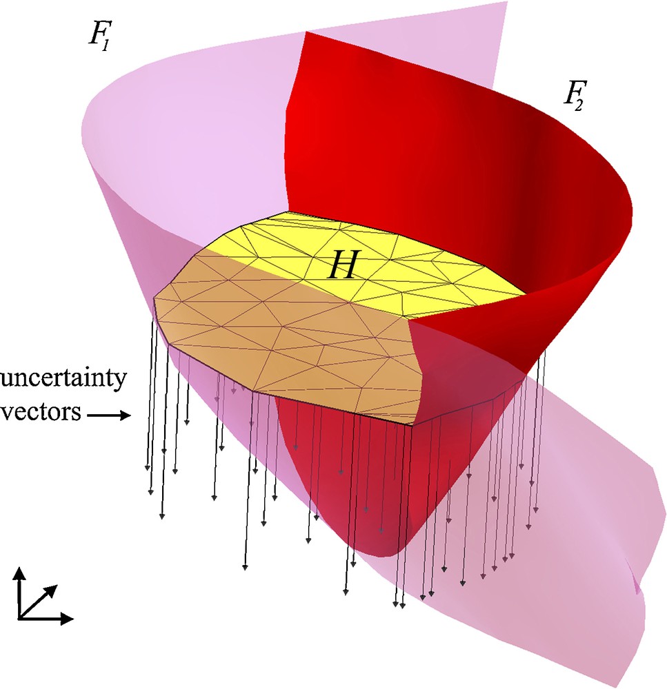
Topology changes induced by geometrical changes. In the reference case, the horizon H is in between faults F1 and F2. A simple drift of H along uncertainty vectors may completely change the configuration: H could possibly occur on either side of F1 or F2 and not anymore in between the two faults.
Changements topologiques induits par des perturbations géométriques. Dans le cas initial, l’horizon H se situe entre les failles F1 et F2. Une simple translation de H le long de vecteurs d’incertitude peut complètement changer la configuration : H pourrait être en contact avec seulement F1 ou F2 et ne plus se situer entre les deux failles.
2.2 Topological perturbation
Topology is all about connections and relations between objects. In a structural model, topological changes may be introduced in different manners:
- • adding or removing geological objects;
- • in the case of faults, changing the truncation rule between two faults;
- • during geometrical perturbations, a simple drift of an horizon along uncertainty vectors may induce a topological change (especially fault to horizon connections, Fig. 1).
Few methods have been proposed to change the topology of a structural model. A fault modeling tool, referred to as Havana, has been proposed in Holden et al. (2003) and Hollund et al. (2002). It is mainly designed for the oil industry and works directly on a corner-point reservoir grid used for flow simulations. This choice allows for directly observing the effects of structural uncertainties on flow simulations. However, resevoir grids have known shortcomings to accurately represent geological structures. Consequently, sub-seismic faults are added by simply modifying the permeability field. Main faults are bilinear planes parallel to the pillars of the reservoir grid or stair-stepped faults.
In our approach, we borrow the idea of fault operator from Holden et al. (2003), but use a flexible representation of faults. This makes it possible to account for large structural uncertainties without making simplifications due to the grid orientation. For accuracy, this method uses an implicit representation of structural interfaces, as in Calcagno et al. (2008), Frank et al. (2007) and Guillen et al. (2008).
2.3 Implicit modeling: new perspectives for 3D modeling
An implicit surface (e.g. Fig. 2d) is described by an isovalue f of a monotonic volumetric function
| (1) |
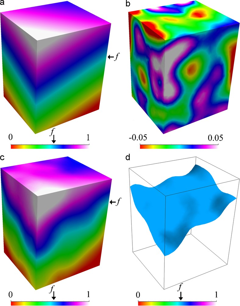
Geometrical perturbation method in implicit modeling. a: the reference scalar field
Geometrical perturbation method in implicit modeling. a: the reference scalar field
Méthode de perturbation géométrique en modélisation implicite. a : le champ scalaire de référence
A conforming stratigraphic column is then represented as a set of isopotentials of a same scalar field, whereas unconformities and faults are defined by their own scalar field. Consequently, horizons can be perturbed independently of faults. Truncations by faults are only honored when an explicit surface is extracted from an isovalue of a scalar field.
Implicit modeling provides a means to easily truncate some surfaces by others using Constructive Solid Geometry (CSG) concepts. For instance, a surface
| (2) |
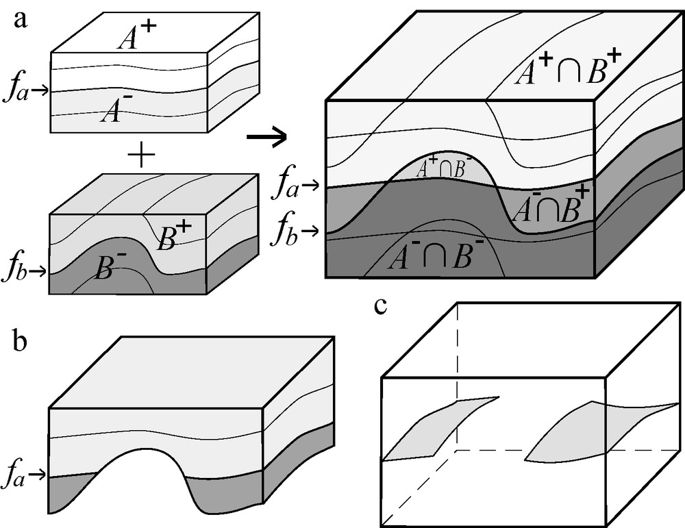
Boolean operations in implicit modeling. a: left: two surfaces
Boolean operations in implicit modeling. a: left: two surfaces
Opérations booléennes en modélisation implicite. a : gauche : deux surfaces
Opérations booléennes en modélisation implicite. a : gauche : deux surfaces
The reference scalar field of an implicit surface
3 A new method for stochastic simulations of fault networks
The proposed stochastic fault simulation method takes advantage of the implicit surface perturbation and CSG operations between faults. To represent how faults partition the domain and interact one with another, we propose using a binary tree.
3.1 Binary trees as descriptors of fault relationships
Indeed, each fault divides the model M in two distinct fault blocks B− and B+ (Tertois and Mallet, 2006), defined by:
- •
- •
Then, in the binary tree representing a fault network, each node represents a fault and each leave (node without children) represents a fault block (Fig. 4).
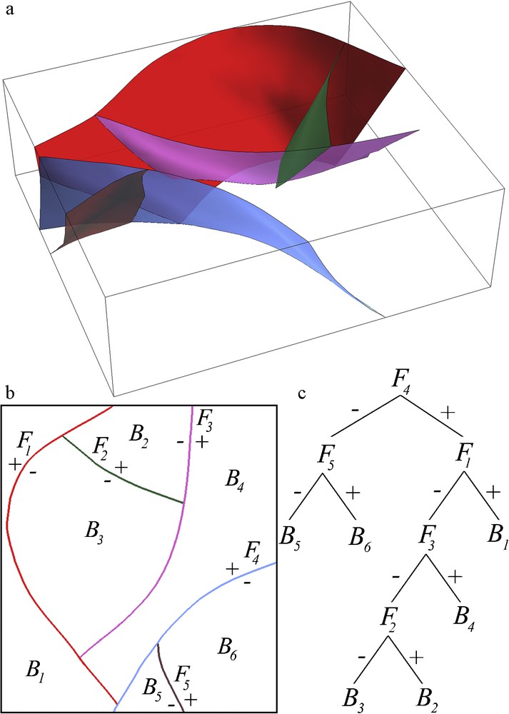
A fault network and its topological representation as a binary tree. a: fault network in 3D; b: the same model in top view to make the topology more explicit. Each fault Fi divides the model in two blocks Bi; c: binary tree representing the fault relationships. The fault F4 is the main and oldest fault (root node of the tree), other faults are branching faults.
Un réseau de failles et sa représentation topologique en arbre binaire. a : réseau de failles en 3D ; b : le même modèle vu de dessus, afin d’expliciter la topologie. Chaque faille Fi coupe le modèle en deux blocs Bi ; c : arbre binaire représentant les relations entre failles. La faille F4 est la faille principale et la plus ancienne (racine de l’arbre), les autres failles étant des failles secondaires.
Each fault in the tree is potentially a branching fault for its parent faults in the tree. Switching a parent and its child in the tree changes their relationship: the main fault becomes the branching fault and inversely (Fig. 5). A special case may occur when a fault F cuts a set of older faults Sold = {Fi|i ∈ [1,n]}. In this case, the oldest faults Sold are on both sides of the cutting fault F in the 3D model, hence they appear in the two branches of F in the tree (Fig. 5c).
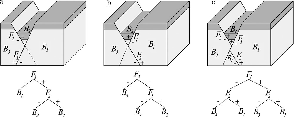
Consequences of filiation relationships in a binary tree from a geological point of view. a: the fault F1 is the root, F2 is a branching fault; b: inversion of the relationship. F1 is now a branching fault; c: a fault F2 being on both sides of F1 means that F2 is cut by F1. F2 is the child of F1 in the tree although it is the oldest fault.
Conséquences des relations de filiation dans un arbre binaire d’un point de vue géologique. a : la faille F1 est la racine de l’arbre, F2 est la faille secondaire ; b : inversion de la relation père-fils. F1 est maintenant la faille secondaire ; c : une faille F2 présente des deux côtés de F1 signifie que F2 est recoupée par F1. F2 est le fils de F1 dans l’arbre bien qu’elle soit plus ancienne.
When modeling a given fault array, some faults may not be truncated by other faults. Therefore, individual faults can be considered either parent or child in the binary tree, there is no consequence in terms of truncation since faults are not in contact. Consequently, a given fault network may be described by several binary trees (Fig. 6). As there is no one-to-one correspondence between a fault network and a binary tree, the latter should be considered as a hierarchy of fault events, the oldest fault being the root of the tree, except for faults offset by more recent faults. Nevertheless, a tree fully defines the topology of the fault network.
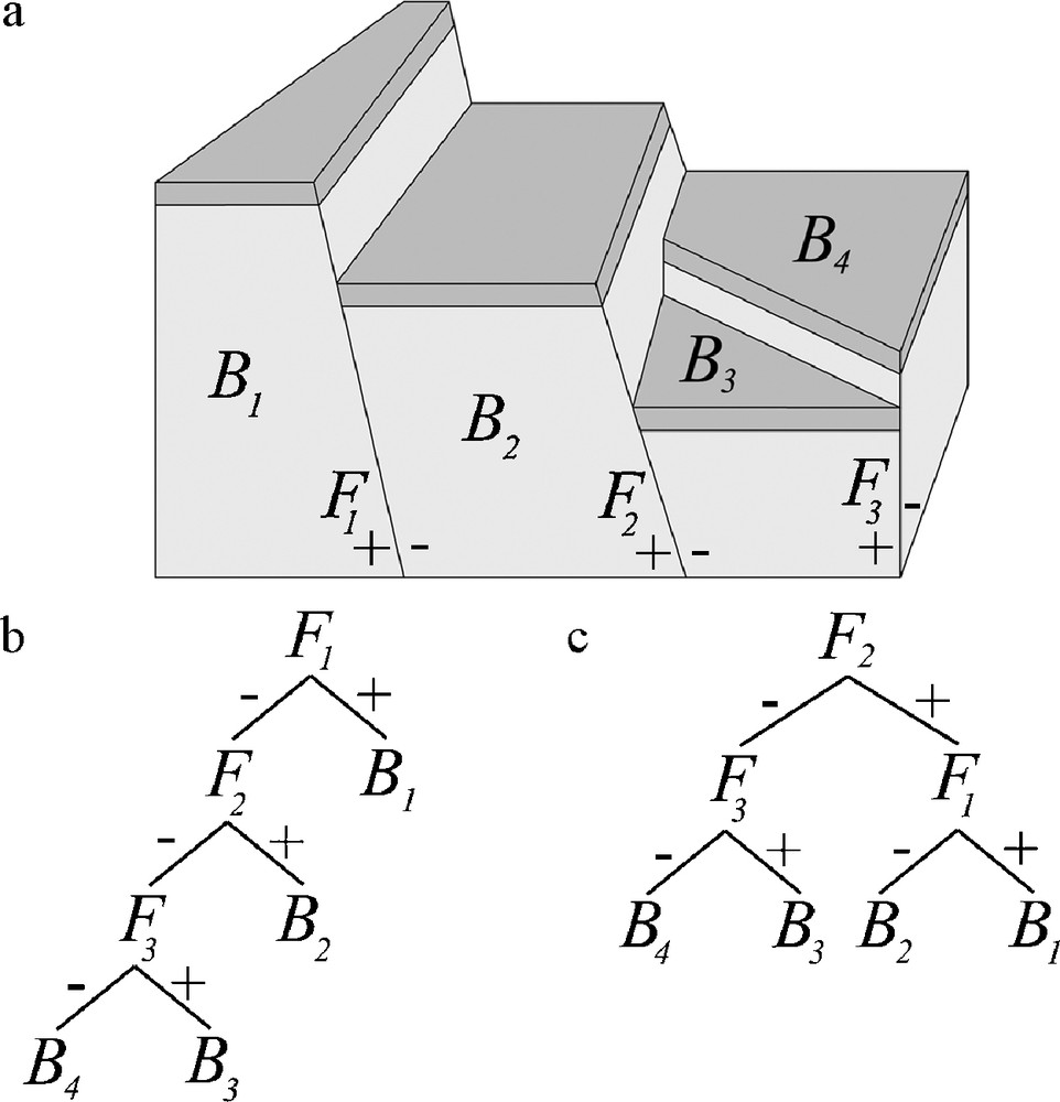
Non-uniqueness of the representation of a fault array in a binary tree. a: 3D diagram representing three faults. The faults F1 and F2 are not in contact so they can either be parent or child in the binary tree; b: representation of the three faults in a binary tree with F1 as the parent fault; c: F2 is now the root of the tree without any change about truncation in the diagram. There may be a consequence of the change deeper, outside the diagram. Masquer
Non-uniqueness of the representation of a fault array in a binary tree. a: 3D diagram representing three faults. The faults F1 and F2 are not in contact so they can either be parent or child in the binary ... Lire la suite
Non-unicité de la représentation d’un ensemble de failles dans un arbre binaire. a : diagramme 3D représentant 3 failles. Les failles F1 et F2 ne sont pas en contact. Par conséquent, elles peuvent être père ou fils dans l’arbre binaire ; b : arbre binaire avec F1 en tant que faille parente ; c : F2 est maintenant la racine de l’arbre, mais aucun recoupement n’a changé. Il se peut que le recoupement change plus en profondeur, en dehors du diagramme. Masquer
Non-unicité de la représentation d’un ensemble de failles dans un arbre binaire. a : diagramme 3D représentant 3 failles. Les failles F1 et F2 ne sont pas en contact. Par conséquent, elles peuvent être père ou fils dans l’arbre ... Lire la suite
3.2 Fault array simulations
3.2.1 Fault network composition
We consider a fault network composed of one or several fault families. Fault families regroup faults having similar structural parameters (orientation, type). If only a few data about a fault family is available, it can be described by statistical input parameters:
- • a relative age;
- • a number of faults;
- • orientation (dip and strike) distributions;
- • perturbation parameters.
Alternatively, fault families may be described by any scalar field (e.g. coming from the interpolation of field, borehole or seismic data) and perturbation parameters defining the associated uncertainties. The key input parameter is the relative age of faults since it determines the order of simulation and thus the place in the binary tree (Section 3.2.3).
To simulate a fault array, only one binary tree is needed, containing all the faults of the network. Different fault networks are obtained by generating different binary trees.
3.2.2 Method for simulating a fault
For a given fault family, each fault is simulated as follows:
- • add a leaf randomly in the tree (i.e. choose randomly a fault block);
- • define the initial fault surface by a reference field
- • perturb the initial geometry by simulating a noise
- • define the fault by the field
- • draw an isovalue f from the range of values that occurs in the selected block to define the fault by
For a model
| (3) |
Using this strategy, no block is priviledged and fault blocks totally different in volume may be obtained. Another strategy consists in balancing the probability by the volume Vi of the block Bi:
| (4) |
The volume of a block defined by several implicit faults can be calculated using the method presented in Royer (2005).
Once a block Bselected has been drawn, an isovalue f corresponding to the fault
3.2.3 Order of simulation
In the general case, fault families are simulated in chronological order, the oldest one first. Consequently, all the faults belonging to the same family are branching faults for the faults belonging to older families (Fig. 7).

Steps for generating a fault network. a: two faults belonging to the same family and the corresponding tree have been simulated. Two faults belonging to another fault family remain to simulate; b: one leaf of the tree is drawn depending on the random function used (e.g. uniform, balanced by block's volume). Once a block is selected, the algorithm generates a field for the next fault and perturbs it using the method presented in Fig. 3. Then, an isovalue is drawn among the range of values present in the selected block; c: the same process is repeated to add another fault. Masquer
Steps for generating a fault network. a: two faults belonging to the same family and the corresponding tree have been simulated. Two faults belonging to another fault family remain to simulate; b: one leaf of the tree is drawn depending ... Lire la suite
Étapes de la génération d’un réseau de failles. a : deux failles appartenant à la même famille ainsi que l’arbre binaire correspondant ont déjà été simulés. Deux failles appartenant à une autre famille doivent encore être ajoutées ; b : un bloc est tiré selon une fonction aléatoire (ex., uniforme, proportionnelle au volume des blocs). Une fois le bloc sélectionné, un champ scalaire est simulé pour la prochaine faille en utilisant la méthode présentée en Fig. 3. Une isovaleur est ensuite tirée parmi les valeurs présentes dans le bloc ; c : le même procédé est répété, afin d’ajouter une faille supplémentaire. Masquer
Étapes de la génération d’un réseau de failles. a : deux failles appartenant à la même famille ainsi que l’arbre binaire correspondant ont déjà été simulés. Deux failles appartenant à une autre famille doivent encore être ajoutées ; b : un bloc est ... Lire la suite
3.2.4 Case of cogenetic faulting
Faults with different structural characteristics (i.e., belonging to different families) may initiate simultaneously at the geological time scale and thus truncate each other. One example of such a situation are conjugate faults, corresponding to steeply opposed-dipping faults. In this case, fault families cannot be simulated one after the other. Instead, let be Scoeval the set of all the faults to be simulated belonging to cogenetic families. The method is iterative: a fault is drawn in the set Scoeval and added randomly in the binary tree, until Scoeval is empty. Consequently, faults belonging to a given family may be parent or child for the other cogenetic families, hence different truncation rules between families (Fig. 8d).
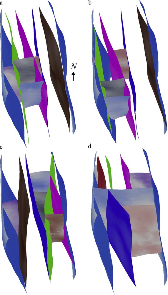
Simulation results illustrating different levels of structural uncertainties in a vertical fault zone. a–b: low uncertainty, only the geometry of fault surfaces is uncertain, the connectivity is fixed; c–d: large uncertainty, both the geometry and the connectivity are uncertain. In c, the fault family oriented north-south is the main family, the second fault family oriented east-west is branching on the first family. In d, even the faulting events are uncertain, fault families are considered as cogenetic families. Masquer
Simulation results illustrating different levels of structural uncertainties in a vertical fault zone. a–b: low uncertainty, only the geometry of fault surfaces is uncertain, the connectivity is fixed; c–d: large uncertainty, both the geometry and the connectivity are ... Lire la suite
Résultats de simulation illustrant différents niveaux d’incertitude dans une zone de faille verticale. a–b : faible incertitude, seule la géométrie des failles est incertaine, la connectivité est fixe ; c–d : incertitude importante, la géométrie ainsi que la connectivité des failles sont incertaines. Pour le cas c, la famille de faille orientée est-ouest est secondaire par rapport à la famille de faille orientée nord-sud. Pour le cas d, l’ordre chronologique des deux évènements de fracturation est incertain, ce qui revient à considérer les deux familles de faille cogénétiques. Masquer
Résultats de simulation illustrant différents niveaux d’incertitude dans une zone de faille verticale. a–b : faible incertitude, seule la géométrie des failles est incertaine, la connectivité est fixe ; c–d : incertitude importante, la géométrie ainsi que la connectivité des failles ... Lire la suite
3.2.5 Case of cross-cutting faults
A special situation may occur when a fault is offset by other faults (Fig. 5c). Indeed, in this case, the parent fault in the tree is the youngest one. This situation can be obtained by simulating the youngest fault Fyoung (Fyoung(x,y,z) = fyoung) first and then simulating the shifted fault Fshifted in a block (adding it at one leaf as usually). Then, depending on the displacement of the cutting fault fyoung, Fshifted may be added to another leaf. Assuming no rotation of fyoung's displacement, Fshifted is defined by the same scalar field but by different isovalues depending on the fault block:
- • Fshifted(x,y,z) = f−|Fyoung(x,y,z) ≥ Fyoung
- • Fshifted(x,y,z) = f+|Fyoung(x,y,z) ≥ Fyoung
4 Perspectives and conclusion
We have introduced a new framework for modeling structural uncertainties. In particular, the method goes beyond the perturbation of deterministic 3D structural interpretations, but considers the uncertainty about connectivities between structural interfaces (Fig. 8). We expect this method to provide a basis for further advances in subsurface uncertainty management, including:
- • taking into account additional data, e.g. field and seismic data, size distribution, slip information. In the case seismic data is available, the global vertical displacement is known for the fault zone. The sum of the simulated displacement for all the faults present laterally in the zone must be equal to the displacement known from seismic data. Some work has also to be done to underline the correlation between the displacement of a fault and its size (Gillespie et al., 1992; Walsh and Watterson, 1988). Such correlations could be used either to simulate the displacement or laterally dying and synsedimentary faults, depending on the available data;
- • how to model particular fault zones? Using our method, realistic fault arrays are obtained but not particular configurations. One may want to simulate, e.g. a fault relay zone, for there is evidence such a structure occurs in the studied area although uncertainties remain. For instance, the probability of a breaching fault to connect two segments of a relay zone must only be defined for the block in between the two segments. It means that some blocks cannot be selected during the simulation, i.e. the binary tree structure is constrained;
- • flower structures between two faults is another challenge since in this case, each fault is both parent and child of the other fault, corresponding to cycles in the tree. To solve this problem, the geometry of a flower structure may be obtained by considering one main fault depending on the sliding direction and an inactive lentil bounded to the sliding surface (Walsh et al., 1999).
The method takes advantage of implicit modeling for both topology description and changes. Each fault is fully described by a monotonic volumetric function
A binary tree has been introduced to describe the spatial relationships between faults. The tree should be considered as a descriptor of fault events, a fault being a branching fault for its ascending branch in the tree. During the fault simulation, faults are added in the tree according to their relative age in order to obtain a fault network honoring input structural constraints. Fault arrays with different topologies are obtained by simulating different binary trees.
Such a multi-realization approach enables to assess the inherent uncertainties to geological data sets. Existing methods are mostly used in the oil industry to reduce economical risks. However, we believe it has a strong potential in other application fields such as potential field interpretation or seismic waveform inversion.
Acknowledgements
This research was performed in the frame of the gOcad research project. The companies and universities members of the gOcad consortium are acknowledged for their support, as well as Paradigm Geophysical for also providing the Gocad software and API. This is CRPG contribution 2020.

