


 CC-BY 4.0
1. Introduction
Disadvantages of earthquake tomography associated with limited illumination can now be compensated by ambient noise tomography with its flexible virtual source and receiver configurations. Both approaches invert far-field observations of travel time differences, obtained from earthquake seismograms [Tromp et al. 2005; Liu and Gu 2012] or from passive Green’s function reconstructions [Shapiro and Campillo 2004; Sabra et al. 2005], for a model of the velocity structure.
Modern dense seismic arrays support alternative local surface wave speed estimations from noise correlation functions [Lin et al. 2009; Lin and Ritzwoller 2011], which includes the large scale application of the frequency domain spatial autocorrelation (SPAC) method [Aki 1957; Ekström et al. 2009; Ekström 2014] that is otherwise typically applied to local sparse array data [Asten 2006]. Dense arrays can now contain on the order of 1000 sensors, which facilitates the proper sampling of the noise correlation amplitude distribution at near-field distances. At zero lag time, the time domain representation of the spatial autocorrelation field is referred to as focal spot, which contains the same information as SPAC and can be analyzed using the same mathematical tools [Cox 1973; Yokoi and Margaryan 2008; Tsai and Moschetti 2010; Haney et al. 2012; Haney and Nakahara 2014].
Focal spot analysis is used in applications that work with a high sensor density. Focal spots have first been studied in time-reversal experiments in underwater acoustics and medical imaging [Fink 1997]. Noise correlation medical imaging transferred the noise seismology approaches to passive elastography, first using far-field surface waves along muscle fibers [Sabra et al. 2007], later using refocusing shear waves. Different properties of the shear wave focal spot have been analyzed including its cross-section width [Catheline et al. 2008; Gallot et al. 2011], two-dimensional shape [Benech et al. 2013; Brum et al. 2015], and its tip curvature [Catheline et al. 2013], which can all be reconstructed using MRI [Zorgani et al. 2015] and ultrasound [Barrere et al. 2020] speckle tracking methods. Importantly, Zemzemi et al. [2020] demonstrated that the ability to discriminate two objects is not controlled and hence limited by the shear wavelength, but instead by the ultrasonic frequency and the pixel density. In seismology, this corresponds to the array station density.
Hillers et al. [2016] first applied Rayleigh wave focal spot imaging in seismology to image lateral velocity variations in a fault zone environment. As for SPAC, the phase velocity is estimated from the focal spot shape using Bessel function models. Using numerical time-reversal experiments based on a Green’s function calculator for one-dimensional layered media [Cotton and Coutant 1997], Giammarinaro et al. [2023] demonstrated the feasibility to accurately estimate phase velocity and dispersion from noisy focal spots. Results for non-isotropic surface wave illumination showed that the wave speed bias is negligible if the sensors are isotropically distributed, compatible with the SPAC results by Nakahara [2006]. Moreover, the effect of interfering P waves can be mitigated using a data or fitting range around one wavelength. Whereas these results from Giammarinaro et al. [2023] suggest the overall robustness and utility of the focal spot method for seismic imaging applications, most notably because of the increase in depth resolution, the study could not address lateral resolution. Considering that super-resolution can be obtained with tip-curvature measurements [Zemzemi et al. 2020], it is important to assess the effect of the data range on speed estimates from densely sampled seismic focal spots.
Here we study systematically the lateral focal spot resolution using numerical experiments. We perform two-dimensional acoustics simulations to reconstruct the Green’s function from reverberating wave fields (Section 2). The ambient field generated in a chaotic closed cavity [Draeger and Fink 1999] yields results that are equivalent to results from open media noise correlation [Derode et al. 2003]. The obtained Green’s function is identical and is here therefore taken as a proxy for seismic vertical–vertical component Rayleigh wave correlations [Sanchez-Sesma 2006; Haney et al. 2012]. We work with a constant number of grid points and a fixed reference frequency. We implement four test cases and vary the data range or fitting distance rfit to investigate the effect on the resolution of the velocity structure. These cases include a homogeneous control experiment (Section 3.1), an interface between two half-spaces (Section 3.2), circular inclusions (Section 3.3), and heterogeneous or random velocity distributions (Section 3.4). In Section 4 we discuss the different resolution aspects that are investigated with the variable configurations for a comprehensive evaluation of the seismic Rayleigh wave focal spot imaging performance.
2. Method
2.1. Synthetic experiments
This study is based on synthetic diffuse wave fields generated in a closed cavity. The resulting correlation functions are equivalent to noise correlations in open media [Derode et al. 2003]. Simulations are performed using the function kspaceFirstOrder2D from the MATLAB toolbox kWave [Treeby et al. 2018]. This function solves a system of first-order acoustic equations for the conservation of mass and momentum using a wavenumber k-space pseudospectral method. The two-dimensional medium is composed of 500 × 500 grid points that are spaced in the x and y direction by dx = dy = 0.1 km (Figure 1a). The background wave speed in the cavity is V0 = 2 km/s. The closed cavity is implemented using different densities outside (𝜌out = 59 kg/m3) and inside (𝜌in = 2950 kg/m3) the cavity. Choosing 𝜌out to be 2% of 𝜌in creates strongly reflecting boundaries from impedance contrast. It supports a homogeneous stability regime of the kWave simulations through a constant Courant–Friedrichs–Lewy number. This number depends on the wave speed, hence varying only the density mitigates potentially problematic stability conditions associated with a large change in wave speed. We cannot exclude the occurrence of weak numerical dispersion in some of the heterogeneous case studies, but the overall consistency of the synthesized Green’s functions and focal spots in the different experiments suggests that this effect does not govern our results. Inside the cavity we select a square target domain consisting of 151 × 151 grid points where we record the solution. In this region we define the different velocity distributions introduced in Section 2.2. Results for each of the four cases discussed in Section 3 are obtained by averaging 11 independent wave field simulations. Each simulation starts with a point source at a different position inside the cavity (Figure 1a). The source term is defined as a time-varying mass source (Figures 1b, c) emitting a 1 s long pulse. The pressure is a differentiation of this signal with the frequency range centered at 1 Hz. The wave field is recorded for 300 s inside the square sub-domain with a 100 Hz sampling frequency.
Configuration of the numerical experiments. (a) Representation of the closed cavity with a background velocity V0 = 2 km/s. The gray area represents the outer part of the medium with the same velocity but with an impedance contrast to trap the waves in the cavity. The red line is the boundary of the closed cavity. The black square indicates the target area where the results are recorded. Inside the cavity the color corresponds to the input wave speed. Red dots indicate the source positions for the 11 realizations. (b) Times series and (c) normalized power spectrum of the emitted pulse used for each simulation. (d) Example of a full time-series recorded in the cavity.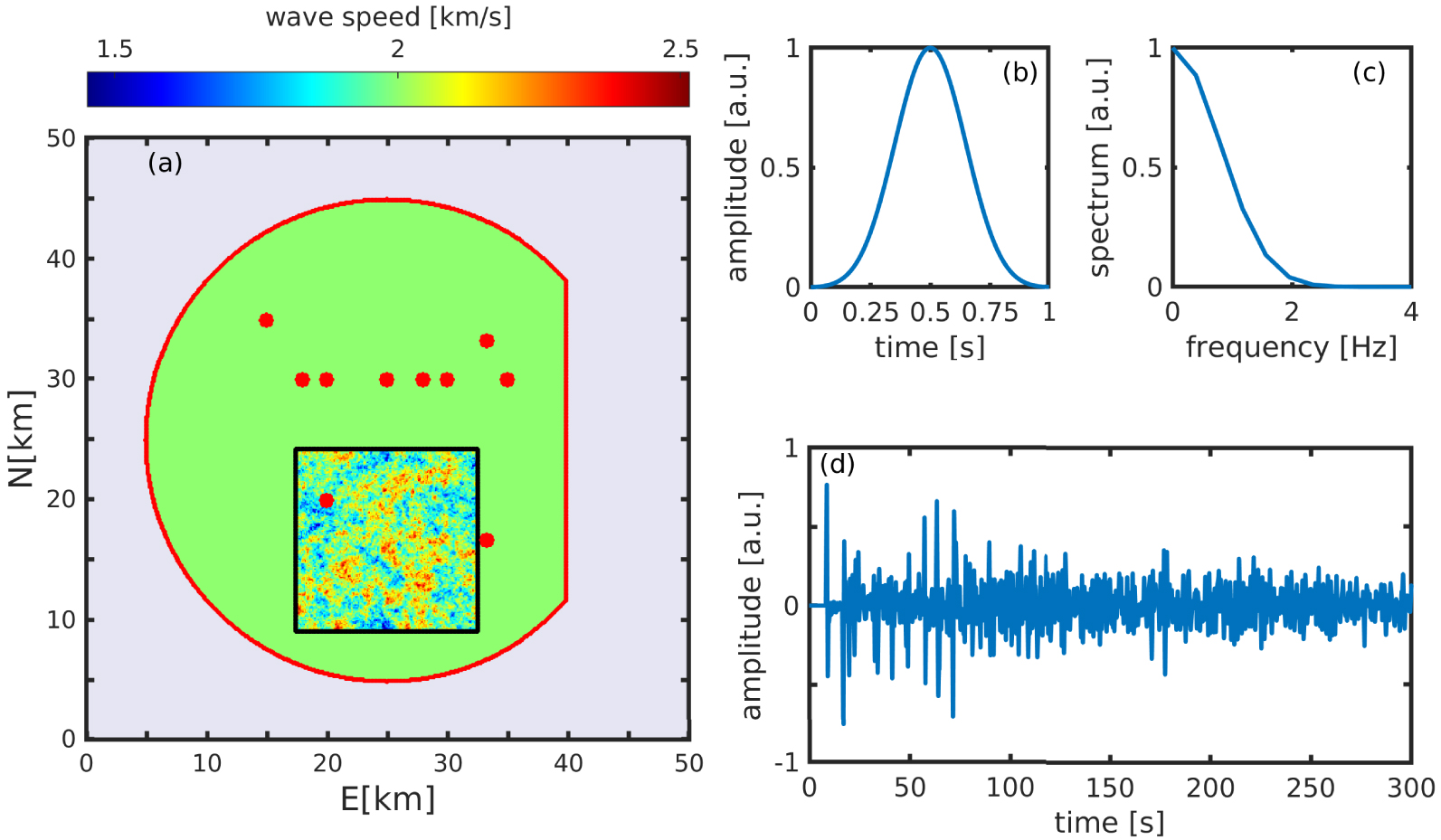
2.2. The acoustic medium in the target domain
The acoustic wave speed distribution V (x) is defined as a spatial function in the square target domain
| (1) |
2.3. Lateral spreading across two welded half-spaces
We modify the homogeneous control experiment and replace the 2 km/s velocity in the left half of the target domain by an increased 2.2 km/s value. This creates two half-spaces and allows us to investigate the lateral resolution as the imaging method induces spreading or averaging across the sharp interface. Such sharp lateral velocity contrasts can occur across bimaterial interfaces in fault zone environments [Weertman 1980; Ben-Zion 1989], or in the contact region of intrusions with the host rock [Chamarczuk et al. 2019].
2.4. Resolution of circular inclusions
Next we perform a classic resolution test and study the power of the method to separate two individual entities in an image. For this we impose three pairs of circular inclusions separated by 0.25𝜆0, 0.5𝜆0 and 1𝜆0. The inclusions have a diameter of 1𝜆0. We test two different sets, where one set of inclusions is stiffer than the background with 𝜉 = 25%, and the other set has more compliant inclusions compared to the background with 𝜉 = −25%. Such a “two-body problem” is typically studied in gel phantom experiments performed in medical ultrasound imaging or medical imaging for tumor detection [Catheline et al. 2013; Zemzemi et al. 2020]. It is a less common configuration in seismology where so-called checkerboard tests are typically employed to quantify the resolution of a tomography configuration. Circular cross-section features can occur in the context of magmatic intrusions or conduits. However, as said, with this configuration we can study the lateral resolution defined as the minimum distance between objects that the method allows to discriminate in an image. This and the other cases are studied using different data ranges rfit discussed in Section 2.6.
2.5. Randomly distributed wave speeds
Last we consider random media using a functional form that is often used to parameterize the heterogeneous distributions of variables such as wave speed, stress, or frictional properties in Earth materials [Frankel and Clayton 1986; Holliger and Levander 1992; Mai and Beroza 2002; Ripperger et al. 2007; Hillers et al. 2007; Sato et al. 2012; Obermann et al. 2016]. We define 𝜉(x) through a spatial 2D inverse Fourier transform as
| (2) |
| (3) |
Parameters for the generation of different heterogeneous media using Equation (3)
| Medium | 1 | 2 | 3 | 4 | 5 | 6 | 7 | 8 | 9 |
|---|---|---|---|---|---|---|---|---|---|
| a (km) | 1 | 1 | 1 | 2 | 2 | 2 | 3 | 3 | 3 |
| 𝜅 | 0.1 | 0.3 | 0.6 | 0.1 | 0.3 | 0.6 | 0.1 | 0.3 | 0.6 |
Where a is the correlation length and 𝜅 governs the sharpness of the spectral decay. The corresponding wave speed distributions are displayed in the top row of Figure 8.
2.6. Data processing and wave speed estimation
Data processing is performed in a Python3.8 environment. For each simulation, we analyze the diffusive parts of the wave field (Figure 2a) by focusing on simulated time series data between 100 s and 300 s (Figure 1d). Considering the distances between the sources and chaotic cavity borders, this corresponds to a range between 10 and 30 mean-free times. We follow Giammarinaro et al. [2023] and filter the traces with a Gaussian filter centered at 1 Hz and with a width of 3.2% to estimate the central frequency dependent phase velocity. In the limit, the analysis could be performed for a harmonic case, however, the narrow filter stabilizes the results. As demonstrated by Giammarinaro et al. [2023], a wider frequency-band filter leads to group velocity estimates, and it biases the focal spot reconstruction by averaging over frequencies which leads to an apparent attenuation. We compute the normalized cross-correlation between each sensor pair to extract the spatial autocorrelation amplitude fields at zero lag time. Results are stacked over the 11 realizations for each case. This yields at short distances around a reference station the large-amplitude feature referred to as focal spot (Figure 2c). The shape is linked to the wave speed through the imaginary part of the Green’s function. From each focal spot we estimate the free parameter wave speed V =𝜔 ∕k by fitting the azimuthal averaged and normalized data to the J0(kr) model using a nonlinear least squares regression algorithm [Hillers et al. 2016; Giammarinaro and Hillers 2022; Giammarinaro et al. 2023]. Again, the 2D acoustic configuration yields results that are equivalent to the lateral propagation of Rayleigh surface waves. The J0(kr) model equally describes the vertical–vertical component of the Rayleigh wave focal spot [Haney et al. 2012; Haney and Nakahara 2014], and V is thus equivalent to the Rayleigh wave phase velocity cR.
Workflow stage examples for the homogeneous medium in the target area. (a) Snapshot of a diffuse wave field. (b) Time-reversed space-time wave field obtained by cross-correlation. (c) Spatial autocorrelation with the focal spot at the center obtained at 1 Hz after stacking over 11 realizations. (d) Simulated 1 Hz focal spot data (gray) and nonlinear regression results for rfit = 0.5𝜆0 (orange) and rfit = 1𝜆0 (red). In this and all subsequent figures the unit 𝜆 is equal to the 1 Hz wavelength 𝜆0 for the reference V0 = 2 km/s.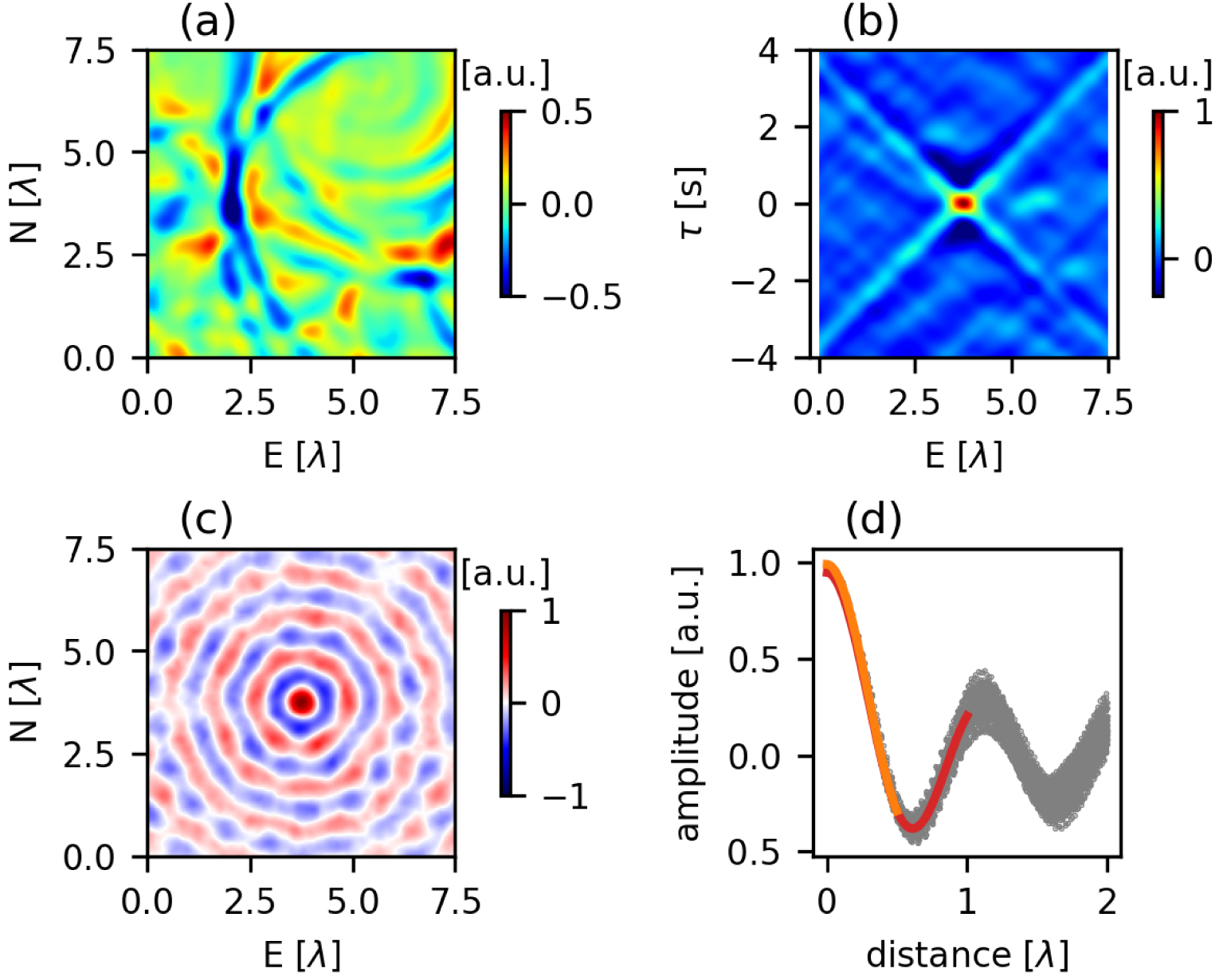
This process is performed for the 22,801 focal spots, and each obtained V estimate is associated with the location of the reference station. This imaging concept thus compiles velocity distributions across dense arrays without solving a tomography inverse problem. Importantly, we choose two different data ranges rfit of 1 km and 2 km associated with 0.5𝜆0 and 1𝜆0 at 1 Hz (Figure 2d). Away from edges, this corresponds to 80 and 314 samples, respectively. We vary rfit because it is a critical tuning parameter, and values around one wavelength yield overall stable results [Giammarinaro et al. 2023]. Larger values can stabilize a regression for noisy signals, but the short distance focal spot imaging concept essentially invites the limitation of rfit for improved resolution. This refers to improved depth resolution as cR values can be estimated at wavelengths that cannot be studied with tomography [Tsarsitalidou et al. 2021; Giammarinaro et al. 2023], but also to the lateral resolution investigated here.
2.7. Error estimation
An important advantage of the focal spot approach is the local assessment of the measurement uncertainty 𝜖 that is estimated following Aster et al. [2019]
| (4) |
| (5) |
3. Results
3.1. The homogeneous reference case
The first test is the homogeneous control experiment which illustrates basic features of the approach. The simulations yield diffuse wave fields that can be used for focal spot imaging. Figure 2(a) shows a snapshot of a diffuse wave field, Figure 2(b) a time-space representation of the time-reversed correlation wave field, Figure 2(c) shows a focal spot of one realization, and Figure 2(d) shows the results of the nonlinear regression following the data processing described in Section 2.6. In Figure 2(b) we can see the refocusing and diverging waves of the Green’s function after cross-correlation. However, the reconstruction is not perfect which is indicated by the small-amplitude fluctuations. The time domain autocorrelation field shows the focal spot at small distances around the origin (Figure 2c). The irregularity of the white zero-crossing contours again illustrates fluctuations and imperfect reconstruction after stacking over 11 realizations. We attribute this to non-perfectly diffuse wave fields associated with the modes in the cavity. However, studies of non-diffuse wave fields [Nakahara 2006; Giammarinaro et al. 2023] demonstrate that isotropically distributed sensors yield unbiased wave speed estimates. This condition is not met along the boundaries of the domain which yields larger fluctuations in the estimates. Figure 2(d) displays results from the nonlinear regression using the two data distances rfit = 0.5𝜆0 and rfit = 1𝜆0. The spread in the data with increasing distance corresponds to the fluctuations from Figure 2(c).
The 2D velocity distributions obtained with rfit = 0.5𝜆0 and rfit = 1𝜆0 are displayed in Figures 3(a) and (b), respectively. The key feature in these images are the speckle patterns. They illustrate that the imperfect reconstruction affects the measurement process to produce these fluctuations around the average reference value. Using rfit = 0.5𝜆0 and rfit = 1𝜆0 leads to V = 2.014 ± 0.034 km/s and V = 2.008 ± 0.021 km/s, respectively, so the V0 = 2 km/s reference value is well recovered with an uncertainty level of 1.5% and 1%. Figures 3(c) and (d) display the spatial error distribution obtained from Equation (5), where the values indicate a similar error range. Both illustrations demonstrate that an increasing data range improves accuracy and precision. Another strong feature are the boundary effects in Figures 3(a) and (b). Recall that we only use observations inside the square target area, similar to an array deployment. The estimation error increases towards the boundaries and the affected area appears to depend on the rfit length. However, the biasing effects are not homogeneously distributed along the boundaries but are largest along the southern edge. This is likely explained by the centered, low position of the target area in the cavity, together with the excitation of specific modes in the cavity that sustain a non-isotropic energy flux in the scattered wave field. This also explains the corresponding pattern of larger uncertainties in the lower half of Figure 3(c). The boundary effects emerge in all our discussed cases but do not affect our conclusions. These effects can be mitigated by a different configuration or geometry, or by averaging over more sources located at more diverse locations.
The control experiment. Focal spot obtained images for (a) rfit = 0.5𝜆0 and (b) rfit = 1𝜆0 for a homogeneous medium with wave speed V = 2 km/s. The reference wavelength 𝜆0 is indicated by the black line and the rfit range used for the nonlinear regression is the radius of the black circle. The indicated wave speeds V are the domain average values and the standard deviation quantify the fluctuations across the domain. Panels (c) and (d) illustrate the spatial distribution of wave speed errors obtained with Equation (5) for rfit = 0.5𝜆0 and rfit = 1𝜆0, respectively.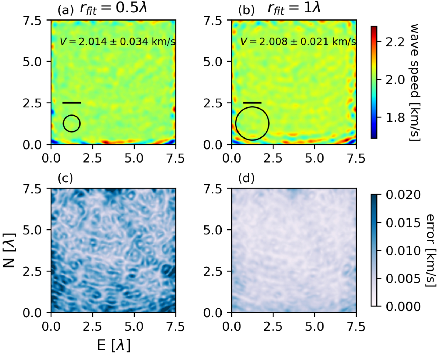
3.2. Resolution of the interface between half-spaces
Figure 4 displays the input wave speed distribution (Figure 4a) and the focal spot-based images of two homogeneous half-space media for the data ranges rfit = 0.5𝜆0 (Figure 4c) and rfit = 1𝜆0 (Figure 4d). As for the control experiment, the distributions show small residual fluctuations around the well resolved input values (the distributions in the left half in panels (c) and (d) yield V = 2.200 ± 0.099 km/s and V = 2.196 ± 0.095 km/s, respectively), and again larger edge effects along the lower boundary.
Results for the two half-spaces. (a) The input model. (b) Reference (blue) and focal spot based velocity profiles obtained with two data ranges (red, black) that are averaged along the N-axis. Panels (c) and (d) show focal spot based images of the velocity. The reference wavelength 𝜆0 is indicated by the black line and the rfit range used for the nonlinear regression is the diameter of the black circle.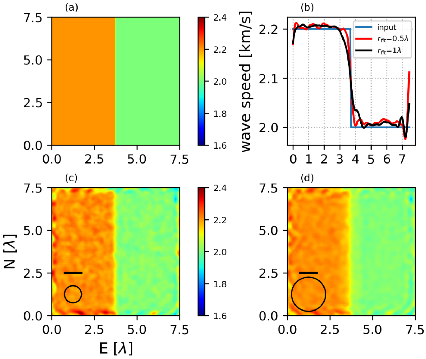
More interesting are the profiles across the domain shown in Figure 4(b). These profiles are averages along the N-axis. The imaged distributions across the interface do not follow the blue input step function but are spread out. To quantify the resolution we estimate the width 𝛥L of the transition. This is the distance between the samples where the amplitude of the estimated profile equals the 5% and 95% values of the 0.2 km/s velocity jump, i.e., when the values are 2.01 km/s and 2.19 km/s. Figure 5(a) enlarges the area around the interface located at 3.75𝜆0. It shows four profiles obtained with rfit values ranging from 0.5𝜆0 to 2𝜆0 in 0.5𝜆0 intervals. It confirms the previous observation that the overall velocity in each half-space is correctly estimated for every data range. As for the results in Figures 3 and 4 we can perhaps discern a weak trend to overestimate the reference values. We attribute this to the imperfect simulation configuration since similar effects are not observed in numerical time-reversal experiments, even in the presence of noise [Giammarinaro et al. 2023]. The width 𝛥L is shown in Figure 5(a) as dotted lines at the bottom, with the vertical dashed lines being the 5% and 95% boundaries of the transition zone. The calculated widths are compiled in Figure 5(b). For rfit = 0.5𝜆0, the transition zone has a width of 𝛥L = 0.4𝜆0. For rfit = 1𝜆0 we obtain 𝛥L = 1.2𝜆0, and for rfit = 2𝜆0, it is 𝛥L = 2.2𝜆0. The spreading effect quantified as the transition width between the two media can hence well be approximated to scale with the data range, 𝛥L ≈ rfit. Figure 5(c) shows the average rfit dependent 𝜖V profiles. The lack of features at the position of the interface indicates that the 10% velocity contrast does not influence the reconstruction. The profiles indicate the tendency of an overall better reconstruction in the right slower domain. This is likely controlled by the proportionally smaller data range in the left faster domain, which is a consequence of the constant rfit value tied to the reference wavelength in the right domain. As expected, this trend weakens with increasing rfit. Figures 5(a) and (c) together show that an increasing rfit leads to a generally increased precision as 𝜖V decreases, but to a loss in accuracy around the position of the interface.
The dependence of the transition width 𝛥L on the data range rfit. (a) Averaged input and imaged wave speed profiles using four different data ranges. Averaging is performed along the N-axis. The vertical dashed lines indicate the location where the amplitudes of the empirical profiles equal the 5% and 95% values of the 0.2 km/s velocity jump. The dotted lines indicate the estimates of the transition width 𝛥L. (b) The transition width 𝛥L as a function of the data distance. (c) The averaged error estimate 𝜖V. Colors in all panels correspond to the same rfit values.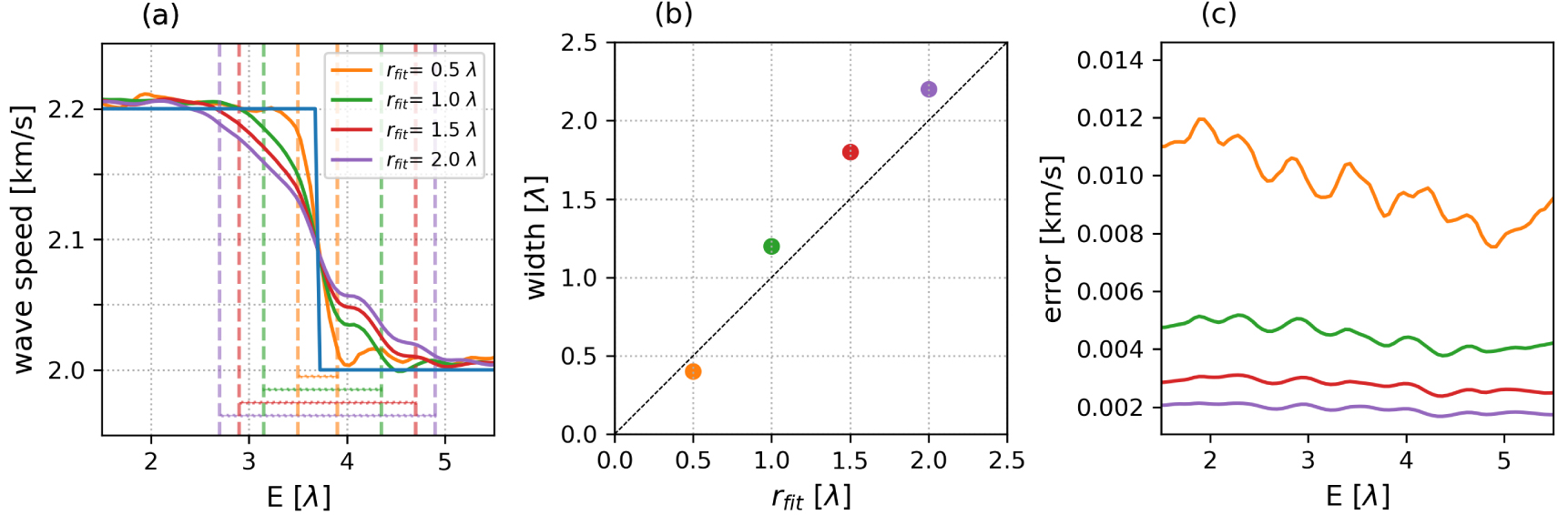
3.3. Resolution and contrast of circular inclusions
We now examine the resolution of pairs of 1𝜆0-wide circular inclusions separated by variable distances. The velocity in the inclusions increases and decreases by 0.5 km/s with respect to the background reference V0 = 2 km/s. Nonlinear regression of the focal spot data are performed using data ranges rfit = 0.5𝜆0 and rfit = 1𝜆0. Figure 6 collects in the left two columns the input wave speed distributions, and the focal spot obtained images for rfit = 0.5𝜆0 and rfit = 1𝜆0. As a general observation, every inclusion is visible on the images for both data ranges, and for the three different distances separating the inclusions. This highlights the effectiveness of the Rayleigh wave focal spot method for “discovery mode” applications [Tsai 2023]. However, the contrast—the difference in “velocity amplitude”—depends on the data range. Using rfit = 1𝜆0 increases the area of the biased velocity estimates. The quantitative aspect of the method decreases with an increase of the data range, which appears as an averaging effect, consistent with the observations across the interface in the half-space case. Panels in the right two columns in Figure 6 show the data from Figures 6(a) to (f) normalized by the input wave speed maps (Figures 6a, b). The overall neutral or white backgrounds illustrate the well resolved reference value. The fact that circular features are visible in Figures 6(i) to (l) demonstrates that the velocity estimates around the edges are biased. The width of the halo or 𝛥L scales again with the data distance, the reconstruction benefits from smaller rfit values (Figures 6i, j).
Results of the circular inclusion resolution test. The left two columns panels (a–f) show absolute values, the right two columns panels (g–l) show scaled values. (a,b) Input models of the three circular inclusion pairs separated by 1𝜆0, 0.5𝜆0, and 0.25𝜆0. The inclusion diameter is 1𝜆0. Focal spot images obtained with (c,d) rfit = 0.5𝜆0 and (e,f) rfit = 1𝜆0. (g,h) Normalized input wave speed map. (i,j) Images in panels (c,d) scaled by the corresponding input distributions in panels (a,b). (k,l) Images in panels (e,f) scaled by the corresponding input distributions in panels (a,b). In the lower two rows, the reference wavelength 𝜆0 is indicated by the black line and the rfit range used for the nonlinear regression is the diameter of the black circle.
These interpretations are supported by wave speed profiles across the inclusions (Figure 7), which demonstrate again that the focal spot image quality, i.e., resolution and contrast, depends on the data range. Inclusions separated by 0.25𝜆0 (Figures 7a, b) are well imaged for small rfit = 0.5𝜆0. The wave speed value away from an interface is well approximated. This applies to the stiff and the compliant inclusions. For rfit = 1𝜆0 the contrast cannot be recovered, which is linked to the data range dependent transition zone width that is here similar to the inclusion diameter. The same mechanism applies to the results obtained with rfit = 1.5𝜆0. Importantly, two inclusions can always be discriminated when the separation distance is 0.25𝜆0, which is yet more obvious from Figure 6. For a separation distance of 0.5𝜆0 this quality of the imaging approach increases, and inclusions are completely discriminated for a distance of 1𝜆0. Taken together, the data range dependent sensitivity of the resolution mostly affects the contrast estimate, but less so the ability to discriminate two objects. The power to discriminate inclusions separated by only 0.25𝜆0 suggests that the property of super-resolution applies, similar to focal spot medical imaging results obtained with ultrasound wavelengths [Zemzemi et al. 2020]. Focal spot imaging resolution thus benefits from high station density across short data ranges. The wave speed estimates are, however, sensitive to noisy data at short distances. In turn, longer data distances reduce fluctuations, which leads to a trade-off between accuracy or contrast and resolution or discrimination [Giammarinaro et al. 2023].
Cross-sections through the circular inclusions. Profiles of input (blue) and estimated wave speeds for rfit = 0.5𝜆0 (orange), rfit = 1𝜆0 (green), and rfit = 1.5𝜆0 (red) for each pair of the circular inclusions. Results are obtained along the E-axis passing through the center of the inclusions. (a,b) Inclusions separated by 1𝜆0. (c,d) Inclusions separated by 0.5𝜆0. (e,f) Inclusions separated by 0.25𝜆0.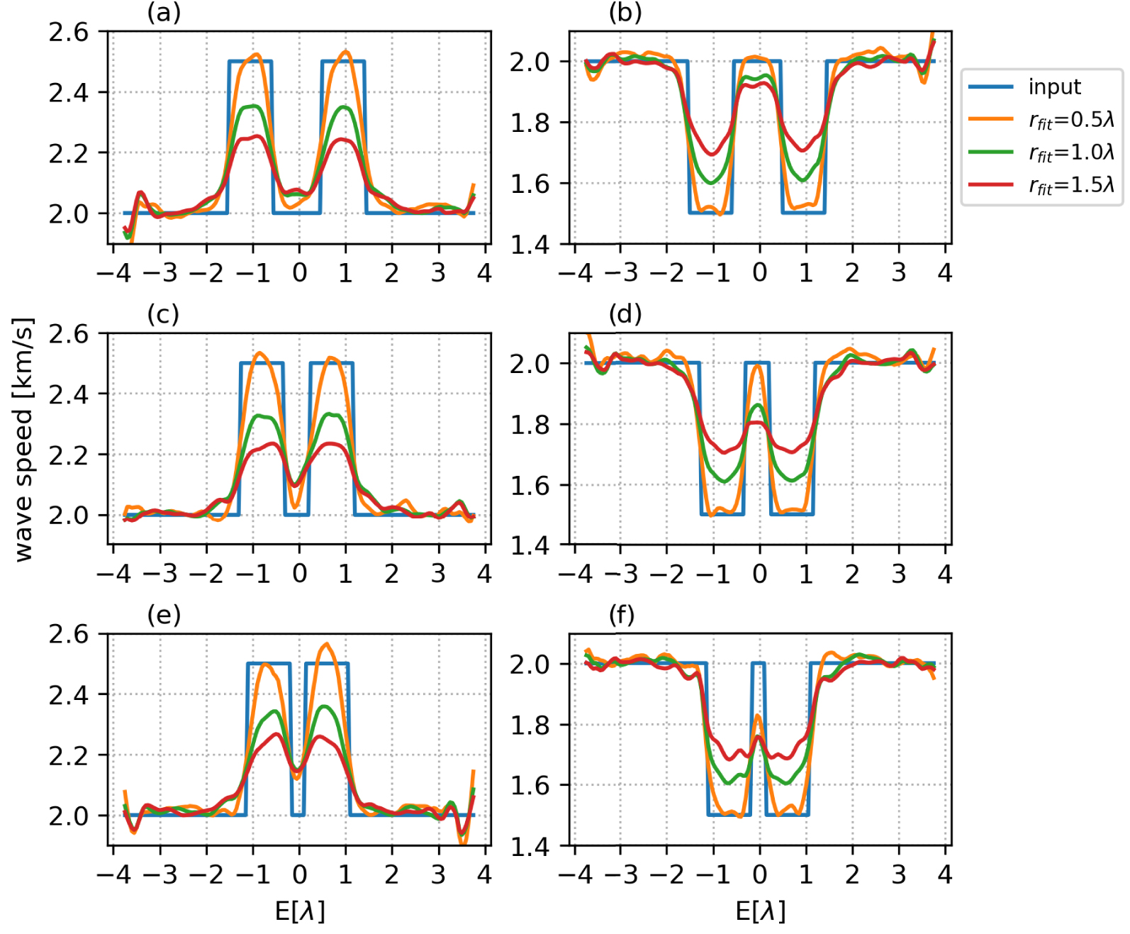
3.4. Imaging random media
The last experiment explores focal spot imaging results of heterogeneous media that are characterized by a von Karman spectral density probability function (Equations (2), (3)). Figure 8 shows input wave speed distributions and the images obtained with data ranges rfit = 0.5𝜆0 and rfit = 1𝜆0 together with the input-normalized images and the formal uncertainties obtained with Equation (5). For each case, we calculate a coefficient of correlation R between the input distribution and the image. As in the previous experimental configurations, the overall pattern of the velocity variations is well retrieved. Peak R correlation values are obtained at zero-lag, which implies no systematic phase change and hence the effectiveness of focal spot “inference-mode” imaging [Tsai 2023]. The smallest coefficient of correlation is R = 0.66 for the small scale, high contrast wave speed variation Medium 1 (a = 0.5𝜆0, 𝜅 = 0.1) and the longer data range rfit = 1𝜆0. The best estimation is obtained for Medium 9 (a = 2𝜆0, 𝜅 = 0.6) imaged with rfit = 0.5𝜆0, which corresponds to analysis using shorter ranges than the correlation length a. This leads to a high coefficient of correlation R = 0.97. Increasing rfit to 1𝜆0 yields R = 0.95. This again confirms our previous results, the images become smoother with increasing rfit, which is synonymous with a loss in contrast and hence details. As an example, in row 6, the green 45-degree trending feature around position x = 3𝜆, y = 2.5𝜆 illustrates a narrow low-velocity zone that is overestimated by the averaging, longer rfit = 1𝜆0. The other way around, the smoother the input distribution for larger a and 𝜅 (Medium 3, 6, 9), the better is the estimate. The corresponding normalized results in rows 3 and 6 illustrate the imaging quality in a complementary style. Predominantly neutral distributions indicate overall good reconstructions, the red-green pattern amplitude range indicates the loss in accuracy, and the color-speckle size is related to rfit. As an example, in row 6, the green 45-degree trending feature around position x = 3𝜆, y = 2.5𝜆 illustrates a narrow low-velocity zone that is overestimated by the averaging, longer rfit = 1𝜆0. The spatial variations of the formal uncertainty estimates in row 4 indicate a medium and wave field dependence. As for the control experiment (Figure 3c) the generally larger error in the lower region is governed by the configuration (Figure 1). The resolution of the comparatively large error spot at x ≈ 6𝜆, y ≈ 3𝜆 in the short correlation length media 1 to 6 highlight the advantage of the local error estimation. Again as for the control experiment, the larger data range in row 7 reduces the uncertainty associated with fluctuations significantly.
Results from the random media case. The top row shows the heterogeneous velocity distributions that are synthesized using Equations (2) and (3). Values of the corresponding tuning parameters are given in Table 1. Rows 2–4 and rows 5–7 show focal spot based results obtained with rfit = 0.5𝜆0 and rfit = 1𝜆0, respectively. For each case, the top rows 2 and 5 show the estimated wave speed distributions, the center rows 3 and 6 show the ratio between the estimated and the input wave speed, and the bottom rows 4 and 7 show the local wave speed error estimates. For each panel, the vertical axis and the horizontal axis correspond respectively to the North and East axis, scaled by the mean input wavelength. The R coefficient is the correlation between the input and the estimated map.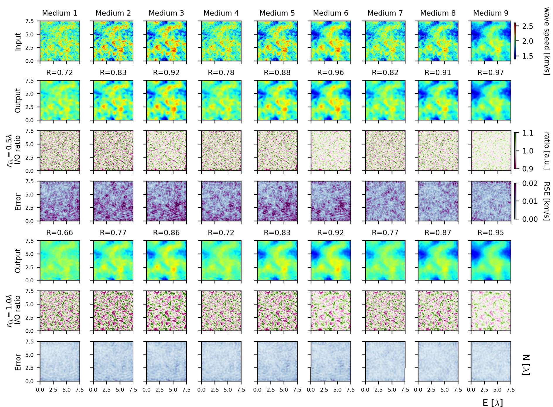
We estimate the relative wave speed change 𝜉 from the wave speed images by inverting Equation (1)
| (6) |
Histograms of the relative wave speed change 𝜉 for the nine media imaged in Figure 8. Blue data correspond to the input reference values, and orange and green data correspond to images obtained with rfit = 0.5𝜆0 and rfit = 1𝜆0, respectively.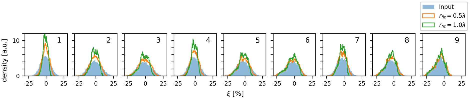
4. Discussion
Resolution can mean different things in different imaging contexts, including the number or density of measuring points, the spectral sensitivity of an imaging device or method, the ability to detect or discriminate features and to accurately estimate their properties, contrast in brightness or color, or phase fidelity [e.g., Smith 2003]. We use numerical simulations of two-dimensional acoustic wave propagation in a cavity (Figures 1, 2) to investigate the lateral resolution of the focal spot imaging technique for a fixed acquisition system with a constant number of grid points. The increase in depth resolution for such a compact dense array configuration compared to measurements made on traveling seismic Rayleigh surface waves is established by Giammarinaro et al. [2023]. We implement four test cases that together allow us to study the lateral resolution power of Rayleigh wave focal spots reconstructed from vertical–vertical component noise correlation data. Lateral resolution is discussed as the ability to resolve a step function in the material properties, to discriminate and characterize two closely spaced objects, and to measure position, amplitude, and phase of random distributions.
In a first homogeneous control experiment (Figures 2, 3) the reference wave speed is estimated with an error below 2% on average, which includes, however, areas of larger bias associated with edge effects. This average error is larger compared to the focal spot results based on numerical time-reversal experiments, where noise-free synthetics lead to errors in the 0.01% range for vertical–vertical component records and data ranges of rfit = 0.5𝜆0 and rfit = 1𝜆0, and where anisotropic surface wave incidence results in biases in the 0.1% range [Giammarinaro et al. 2023]. The different error levels are associated with the different methods used to synthesize Green’s functions and focal spots. In time-reversal experiments, the wave field and hence the ballistic wave correlations are fully controlled by the mirror properties. More mirror elements lead to better refocusing results. Controlled lab experiments can stack over different space realizations. In seismic data applications an improved Green’s function and refocusing reconstruction is achieved by time averaging to better conform with the decorrelated noise source assumption. Here, the focal spots are retrieved from cross-correlation of the reverberating cavity wave field, where the quality of the Green’s function is controlled by the ability to excite and average a sufficiently large number of modes in the cavity [Draeger and Fink 1999]. Hence we stack over different realizations using different source positions. This increases the number of independent modes to enhance the narrow-band refocusing, which is equivalent to using more time reversal mirror elements in a time-reversal experiment. Our approach converges towards the theoretical focal spot, but it remains sensitive to details of the implementation such as the source positions of the relatively few realizations. This explains the observed fluctuations in the focal spot reconstructions, which indicate the imperfect Green’s function synthesis, even for the homogeneous case. This means that our imperfect cavity results are comparable to focal spots obtained from noisy data.
The second half-spaces experiment (Figures 4, 5) shows the feasibility to resolve the contrast between two media that have a 10% difference in wave speed. However, the interface is not perfectly resolved. Whereas the wave speed is correctly estimated away from the interface, the finite data or fitting range creates an averaging or low-pass filter effect that depends on rfit. Tests with different rfit values indicate that the transition width 𝛥L scales with good approximation linearly with the data range, 𝛥L ≈ rfit.
The third circular inclusion configuration (Figures 6, 7) shows the possibility to discriminate two separate objects separated by 0.25𝜆0, even for data ranges of one wavelength. However, the data range dependent low-pass filter properties lead to averaged amplitude values at edges. We have not observed situations where the focal spot method yields biased phase properties, so the inclusion positions are accurate. This suggests that the super-resolution property demonstrated with passive elastography in soft tissues [Zemzemi et al. 2020] also applies to 2D Rayleigh surface wave propagation. Again this means that for good data quality and high station density the method has the potential to meet the formal criterion of super-resolution, i.e., the sensitivity at small scales is sufficient to discriminate objects or features that are separated by distances that are much shorter than the wavelength.
The fourth test case considers random media (Figures 8, 9, Table 1) which show the highest similarity to distributions of Earth material properties. The quality of the focal spot reconstruction as quantified by the correlation coefficient R between reference and image depends on the roughness or smoothness of the distribution in relation to wavelength and data range. R is small when the distributions are rough, have small-scale fluctuations compared to the probing wavelength, and the data range is large. The reconstruction is almost perfect when the distributions are smooth, have large-scale fluctuations, and the data range is small. These conclusions are further corroborated comparing histogram properties of the velocity variation parameter 𝜉 (Equation (2), Figure 9), which again demonstrate the low-pass filtering effect of large rfit values. Thus, positions are well estimated but the amplitudes diverge for small-scale heterogeneities. The best estimates are obtained for variations on scales larger than rfit. Deblurring methods can potentially be developed to further improve the lateral resolution of the method considering that the focal spot Bessel function shape acts as a spatial convolution filter. If resources permit, an imaging campaign could be optimized by first detecting target features with low contrast before then a sensor re-configuration helps to improve the quantitative estimate by increasing the signal-to-noise ratio through network densification.
The present study employs two-dimensional acoustic simulations. These scalar simulations yield the same Green’s function as for vertical–vertical component Rayleigh wave propagation. Our main conclusions thus hold for seismic Rayleigh wave imaging, including the advantageous estimation of the local error that can help improve the uncertainty management of shear wave inversions. However, this set-up does not allow to study the biasing effect of interfering body wave energy. Giammarinaro et al. [2023] shows that the error on the vertical–vertical component increases in the presence of P waves, but this can be compensated for by increasing the data range. Together with our observations here this implies that an increase in rfit improves the results if refocusing P wave energy distorts the surface wave focal spot, but that this remedy negatively affects lateral resolution power. This trade-off situation would benefit from efficient focal spot filters. Alternatively, Rayleigh wave phase speed estimates obtained from radial-vertical component data are much less sensitive to P waves [Giammarinaro et al. 2023], which offers independent constraints for the improvement of vertical–vertical results. The application of radial–radial and transversal–transversal component focal spots requires first an efficient separation of the combined Rayleigh and Love wave energy [Haney and Nakahara 2014]. Spatial autocorrelations of surface wave strain and rotational data can further provide additional constraints on the local velocity structure [Nakahara et al. 2021; Nakahara and Haney 2022].
5. Conclusion
We investigate the lateral resolution power of the Rayleigh surface wave focal spot imaging method using two-dimensional numerical experiments of reverberating wave fields in a cavity. Most importantly the resolution depends on the data range. This means that focal spot imaging exhibits super-resolution properties provided the data quality supports sub-wavelength data ranges. Longer data ranges still allow imaging of small-scale features at super-resolution albeit with a loss in contrast. Seismic Rayleigh wave focal spot imaging shows convincing resolution properties that make it suitable for a wide range of imaging applications ranging from feature detection to accurate wave speed estimates. There are hence no fundamental disadvantages compared to established passive surface wave tomography methods. Here as there, the station configuration can be tuned to support image quality and properties for different goals, and in both cases the data quality or signal-to-noise ratio ultimately has the largest impact on the resolution.
Declaration of interests
The authors do not work for, advise, own shares in, or receive funds from any organization that could benefit from this article, and have declared no affiliations other than their research organizations.
Open research/data availability
No observational data were used in this study.
Dedication
The manuscript was written with contributions from all authors. All authors have given approval to the final version of the manuscript.
Funding
This work was sponsored by a research grant from the Academy of Finland (decision number 322421).
Acknowledgments
We thank Julien de Rosny, Stefan Catheline, Michel Campillo, Léonard Seydoux, Laurent Stehly, Alexander Meaney, and Markus Juvonen for helpful discussions. We thank the editor N. Shapiro and two anonymous reviewers for comments that helped to improve the manuscript.