


 CC-BY 4.0
1. Introduction
The Alpine mountain range is part of the continental collision ranges created by the convergence of the Eurasian and African plates in the Mediterranean region. It results from the subduction of the Alpine Tethys under the Adriatic microplate since the Late Cretaceous, and the subsequent continental collision between the European and Adriatic paleomargins in the Cenozoic [e.g., Handy et al. 2010]. The Alpine belt is an outstanding example of subduction and continental collision studies, which has been investigated by geologists for more than 150 years. Several major concepts of modern geology have been developed in the Alps, such as nappes, when the prominence of horizontal over vertical displacements was proposed by Emile Argand [Argand 1922]. More recently, the identification of coesite, which is a high-pressure polymorph of quartz, in gneisses of the Dora Maira massif (south-western Alps, Italy) led Chopin [1984] to propose that continental crust may be subducted to depths of 90 km or more. The amount of geological knowledge about the Alps is unparalleled in any other mountain range, and they provide a unique natural laboratory to advance our understanding of orogenesis and its relationship to present and past mantle dynamics. The Alpine mountain belt is also a populated area where millions of Europeans are affected by its topography, geology and associated natural hazards such as earthquakes or landslides. Yet, accurate information on the lithospheric structure of that emblematic and populated mountain range was hampered by insufficient and spatially heterogeneous geophysical data until the last few years. Filling that gap was the primary motivation for the AlpArray initiative, which gathered a large number of European research institutions to deploy a dense and homogeneous temporary broadband seismological network over the Alps and its forelands to complement the permanent networks [Hetényi et al. 2018a].
In addition to gaining knowledge of Alpine lithospheric structure, the high spatial coverage of AlpArray temporary stations and permanent networks has given us the opportunity to develop new methods of seismic tomography at this large regional scale based on ambient noise. A review of these methodological developments is gathered in this paper because they could be applied with great benefit to other similary dense networks.
1.1. Seismic imaging in the Alps
Seismic imaging is an essential complement to geological studies to build lithospheric-scale interpretive models and improve the understanding of the dynamics of the mountain belt in space and time. The geometry and depth of the crust-mantle boundary, only accessible with geophysics and in particular active-source seismology and earthquake seismology, are key information for geological and geodynamic modeling. Each of these methods has limitations and provides partial information, which is why noise-based tomography methods are a valuable complement. In the Alps, deep seismic sounding (DSS) experiments including ECORS-CROP in the Western Alps [e.g., Nicolas et al. 1990], NFP-20 in the Central Alps [e.g., Frei et al. 1990], and TRANSALP in the Eastern Alps [e.g., Lüschen E. et al. 2006] provided crucial data for interpretive crustal-scale sections along a number of crooked lines mostly transverse to the belt. The results from these localised studies cannot be extrapolated to other locations along the belt due to its arcuate, non-cylindrical geometry. DSS profiles provide high-frequency reflectivity images of the crust, hence sharp and sub-horizontal velocity contrasts with no or poor information on absolute velocities. Thus, they cannot be interpreted in terms of petrology. Moreover, the European Moho, defined as the base of the highly reflective lower crust, was not detected below the intensely deformed and highly heterogeneous crust of the internal zones in the ECORS-CROP and NFP-20 W5 and E1 profiles across the Western and Central Alps [e.g., Nicolas et al. 1990; Marchant and Stampfli 1997]. The deep European Moho has only been detected by the ECORS-CROP wide-angle seismic reflection experiment under part of the internal zones to a maximum depth of 55 km [ECORS-CROP Deep Seismic Sounding Group 1989].
A similar type of information on velocity contrasts beneath seismic stations is provided at lower frequencies by receiver function (RF) analysis in particular for Moho depth estimates [e.g., Kummerow et al. 2004; Lombardi et al. 2008; Zhao et al. 2015; Hetényi et al. 2018b; Paul et al. 2022; Michailos et al. 2023]. In some specific cases, such as in the presence of a very heterogeneous, scattering crust, receiver function analysis can be more effective at detecting the crust-mantle boundary than reflection seismics because it uses low-frequency, high-energy waves from teleseismic earthquakes that travel across the heterogeneous crust only once. Moreover, receiver functions computed for station arrays provide estimates of Moho depth with 2-D coverage. Indeed, Spada et al. [2013] generated a Moho depth map of Italy, including the Alpine region, which combines DSS data with receiver functions. Spada et al. [2013]’s model displays three Moho surfaces, European, Adriatic-Ionian and Ligurian–Corsican–Sardinian–Tyrrhenian. As this model allows only one Moho at a given location, the Moho surfaces never overlap, even though the European lithosphere is known to underthrust Adria.
The polarity of converted waves in receiver functions provides useful information on the sign of velocity change with depth. For example, Zhao et al. [2015] observed negative-polarity P-to-S converted waves in RF of the CIFALPS profile close to the so-called Ivrea body positive Bouguer anomaly (blue line in Figure 1). This gravity anomaly high is known since the first geophysical experiments in the Alps that also reported high-velocity refracted waves (Vp = 7.4 km/s) at 10 km depth in the same area of the Italian Piemonte region [Closs & Labrouste 1963]. The source of this gravity and seismic velocity anomaly is called the Ivrea body and it is interpreted as a slice of Adriatic upper mantle at unusually shallow depth [e.g., Nicolas et al. 1990]. The negative-polarity converted phases in the RF of the CIFALPS profile were the first evidence for the inverted Moho beneath the Ivrea body, as the contact between the high-velocity Adriatic mantle wedge on top and the lower velocity European crust or subduction interface below [Zhao et al. 2015]. These negative-polarity converted waves from 20–60 km depth and the positive-polarity conversions at 75–80 km depth were the first seismic evidence for continental subduction of the European lithosphere beneath Adria, according to Zhao et al. [2015]. Like deep seismic sounding, however, receiver functions yield no clues on absolute velocities.
Maps of broadband seismic stations in the Alps and surrounding regions including all stations used in the studies discussed in Sections 2–3; (a) before 2010: red triangles are public permanent stations in 2009; (b) after 2020: red triangles are permanent stations in 2019; green triangles are temporary stations used in the studies described in this paper (EASI, AlpArray, CIFALPS and CIFALPS-2). The blue line in (a) and (b) is the 0 mgal contour of the Ivrea Bouguer anomaly. Black lines: main geological units and faults from the tectonic map compiled by M. R. Handy. The thick black line CC′ is the CIFALPS profile used in Figure 3. DM: Dora Maira massif; IGA: Ivrea gravity anomaly.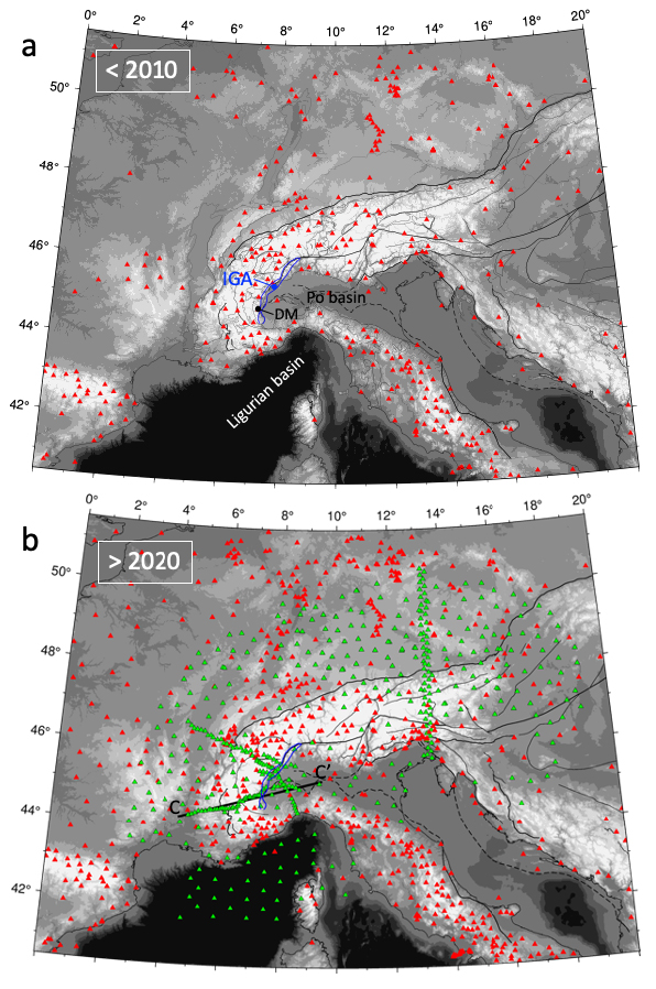
Local earthquake tomography (LET), which relies on the inversion of body-wave arrival times (mostly direct P and S waves) from local earthquakes for absolute velocities (Vp and Vs or Vp/Vs) is an efficient tool to get 3-D images and complement 2-D DSS or receiver function reflectivity images. The size of the imaged crustal volume and the resolution of the tomography depend on the distribution of seismic stations at the surface and earthquake hypocenters at depth. In the Alps, the seismicity level is low to moderate, with rare events of magnitude > 5. Many years of recording are therefore required to reach sufficient ray coverage in local earthquake tomography studies of the whole Alpine region like in Diehl et al. [2009]: 12 years (1996–2007) for 1500 events of Ml > 2.5. Another issue is that most earthquake sources in the Alps are shallow (focal depths < 15 km), except in the westernmost part of the Po basin where hypocenters on the Rivoli-Marene fault reach 70–80 km depth [Eva et al. 2015]. Due to low magnitudes, these deep events are only detected by stations close to epicenters. They, however, proved useful to image the deep parts of the subduction wedge of the western Alps by LET including the high-velocity Ivrea body [Solarino et al. 1997; Paul et al. 2001; Solarino et al. 2018; Virieux et al. 2024]. Imaging the crust to Moho depth with LET in most of the Alps requires records of Pn waves, thus sufficient-magnitude earthquakes and station arrays of large spatial extent. Until recent years, this last condition was only reached by compiling records of a large number of regional and national networks with heterogeneous data sharing policies and traveltime picking strategies, at the cost of heavy homogenization work [13 networks used in Diehl et al. 2009; Bagagli et al. 2022, and Virieux et al. 2024].
In addition to low-to-moderate seismicity and heterogeneous coverage of permanent seismic networks, the strong crustal heterogeneity and its very 3-D character are other challenges in seismic tomography of the Alpine lithosphere. Crustal heterogeneity is not surprising for a collisional belt with a long tectonic history. However, the arcuate shape of the western Alps, the presence of large and deep basins including the Po basin and its unconsolidated sediment layers and high level of anthropogenic noise close to the heart of the belt make seismic imaging of the Alpine lithosphere particularly challenging.
Since Aki et al. [1977], the most basic and often used method to image seismic heterogeneities in the upper mantle is teleseismic tomography. It is based on the inversion of observed relative arrival times of P (or S) waves generated by earthquakes at teleseismic distances (>20°) for relative variations of P (or S) wave velocity (Vp, or Vs) in the upper mantle beneath a seismic array. Teleseismic tomography has been widely used to image fast-velocity slabs interpreted as subducted continental and/or oceanic lithosphere in the Alpine upper mantle [e.g., Lippitsch et al. 2003; Piromallo and Morelli 2003; Zhao et al. 2016a; Paffrath et al. 2021]. Contrasting results of these mantle tomography studies have led to controversies about the geometry of the slabs at depth, including whether the European slab is attached or detached in the western Alps [e.g., Zhao et al. 2016a], or whether Europe is the upper or lower plate in the eastern Alps [e.g., Lippitsch et al. 2003]. These questions are still of the utmost importance to understand the past and present dynamics of the mountain belt. A major issue for teleseismic tomography is the difficulty in separating the contribution of the crust from that of the mantle in arrival times for near-vertical ray paths [e.g., Waldhauser et al. 2002]. This is of particular importance in mountain ranges such as the Alps due to strong changes in crustal thickness.
The mantle structure can also be imaged with teleseismic surface-wave tomography [e.g., El-Sharkawy et al. 2020]. Frequency-dependent traveltime data of surface waves are inverted for S-wave velocity as for ambient-noise tomography, but using periods >30 s. To overcome the poor sensitivity of such long period surface waves to crustal structure, Kästle et al. [2018] have jointly inverted dispersion data from ambient noise correlations in the short-period band (8–30 s) with data from teleseismic surface-wave records at longer periods. The horizontal resolution of the resulting shear-wave velocity models however remains rather low in the upper mantle, limiting the value of this type of model in the debates on slab geometry beneath the Alpine range.
1.2. Ambient noise imaging in the Alps before AlpArray
Ambient noise tomography (ANT) is particularly well suited to imaging the Alpine crust as a complement to the methods outlined in the previous section because (a) it does not require local earthquakes [Shapiro et al. 2005], and (b) the period range of seismic noise is adequate for crustal imaging, in contrast to teleseismic surface wave tomography which is dominated by longer wavelengths. A sufficient coverage of the study region by seismic arrays is the only requirement for a fairly resolved 3-D velocity model since each station becomes a wave source for all other stations in the noise cross-correlation process [Campillo and Paul 2003; Shapiro and Campillo 2004].
Since the first application of ambient noise tomography to the Alps by Stehly et al. [2009], station coverage has improved significantly in density but also in spatial homogeneity. This improvement is due to numerous new permanent broadband stations (in Austria, Germany, France, etc.) and to temporary networks, most importantly the AlpArray seismic network [AASN; AlpArray Seismic Network 2015]. Indeed the AASN, which included more than 600 stations, was designed to fill in gaps between permanent stations and to homogenize spatial coverage in a way that no location in the Alps was more than 30 km away from a seismic station onland [Hetényi et al. 2018a]. The AASN also had a marine component with 29 ocean-bottom seismometers (OBS) deployed for 8 months in the Ligurian basin. It was complemented by denser quasi-linear or 2-D temporary arrays on targets of specific interest. The most important ones were EASI across the Eastern Alps [AlpArray Seismic Network 2014], CIFALPS and CIFALPS-2 across the Western Alps [Zhao et al. 2016b, 2018], and Swath-D in the Central and Eastern Alps [Heit et al. 2017]. Figure 1 shows the seismological stations prior to 2010, and the stations which were used in the studies summarised in this review. For seismic tomography in general, and ambient noise tomography in particular, there is clearly a time before and a time after AlpArray.
Before AlpArray, the limited coverage of large parts of the Alpine area only allowed for ambient noise tomography studies of the central Alps, relying mainly on the dense Italian and Swiss permanent networks [Stehly et al. 2009; Verbeke et al. 2012; Molinari et al. 2015]. The pioneering application of ANT to the Alps by Stehly et al. [2009] used records of 150 broadband stations in Switzerland and neighbouring countries. They applied a classical two-step procedure, with an inversion of dispersion measurements for group velocity maps of Rayleigh waves in the 5–80 s period band, followed by a non-linear Monte Carlo inversion of the dispersion curve in each cell for a 1-D shear-wave velocity model. The set of 1-D models were then merged into a so-called 3-D Vs model that should more properly be called pseudo 3-D. This study provided a data constrained Moho depth map of the Western Alps, because crustal thickness was a free parameter in the inversion. This Moho map shared many similarities with the reference map computed by Waldhauser et al. [1998] from depth-migrated controlled-source seismic data, including strong and abrupt Moho depth changes from 25–30 km beneath the European forelands and the Po plain, to 55 km beneath the internal Alpine arc from southern Switzerland to the Dora Maira massif (Piemonte, Italy). This first successful application of ANT in the Alps was considered a proof of concept. The tomography by Stehly et al. [2009] was followed by those of Verbeke et al. [2012] and Molinari et al. [2015], who expanded the station array to the Italian and Slovenian permanent broadband networks and the tomography to the Apennines, and used both group and phase velocity dispersion data.
In the last large-scale ANT before AlpArray, Kästle et al. [2018] used records of 313 permanent stations covering the broad Alpine region and the Apennines. To overcome the sparse station coverage in the external, western and northern Alps, they complemented ambient noise phase dispersion measurements with two-station measurements from regional and teleseismic earthquake records. The ambient noise and earthquake-based dispersion datasets agreed well enough in the overlapping period band 8–60 s to be jointly inverted for Rayleigh and Love wave phase velocity maps in the broad period range 4–250 s [Kästle et al. 2016]. In a second stage, Kästle et al. [2018] jointly inverted Rayleigh and Love-wave phase dispersion data in each cell for 1-D Vp and Vs models of the crust and upper mantle. According to the authors, the 3-D Vs model of the upper mantle derived from joint inversion has much higher resolution than when each individual dataset, ambient noise and earthquake-based, is inverted alone. By averaging the crustal thickness of the 500 best-fitting Vs models, Kästle et al. [2018] computed a Moho depth map that compares remarkably well with receiver function and DSS Moho depth estimates along numerous profiles across the Alps and Apennines [Kummerow et al. 2004; Spada et al. 2013; Zhao et al. 2015].
The installation of the AlpArray temporary seismic network started in Austria in the summer of 2015 and ∼200 of the planned 267 temporary stations were operating by mid-2016 [Hetényi et al. 2018a]. By adding the first months of AASN recordings (until June 2016) to a four-year noise dataset from European-wide permanent broadband networks, Lu et al. [2018] achieved the first ANT of the broad Alpine region with fairly homogeneous coverage and an average station spacing of ∼50 km. This study was the first in a series of noise-based isotropic and anisotropic tomography studies on the Alpine lithosphere that have built on the spatial homogeneity and density of the AlpArray dataset (from both permanent and temporary stations) to develop and apply new data analysis and imaging methods.
Indeed, the high spatial density of AASN and associated permanent and temporary networks has driven methodological advances in ambient noise tomography, just as the USArray Transportable Array has driven the advent of Eikonal tomography [Lin et al. 2009]. The present paper focuses on key methodological advances on isotropic (Section 2) and anisotropic (Section 3) imaging. We also show how the application of these new methods to Alpine data opens new perspectives (Section 4) for the geological and geodynamic modeling of the Alpine belt.
2. Isotropic ambient noise tomography
The homogeneous coverage provided by the AASN motivated a number of ambient noise isotropic tomography studies on regional targets in and around the Alps [e.g., Guerin et al. 2020; Molinari et al. 2020; Sadeghi-Bagherabadi et al. 2021; Schippkus et al. 2018; Szanyi et al. 2021]. In this section we focus on noise-based isotropic tomography studies of the broad Alpine region and surroundings using all or most available stations in Western Europe at the time of study. We describe three key improvements to isotropic imaging with cross correlations in this highly heterogeneous area.
2.1. Second-order cross-correlation techniques
The Ligurian basin, which separates the Corsica–Sardinia block from the southern coast of France and north-western Italy (Figure 1) is a back-arc basin generated by the rollback of the Adriatic slab in Oligo-Miocene time [e.g., Rollet et al. 2002]. Situated at the transition between the Alps and Apennines mountain ranges, it was considered an important target for the AlpArray temporary seismic experiment, which therefore included 24 broadband ocean-bottom seismometers (OBS, Figure 1).
Ambient noise tomography of an offshore area is possible without OBSs provided that it is surrounded by land stations. For example, Magrini et al. [2022] have computed an S-wave velocity model of the west-central Mediterranean, including the Ligurian basin, from surface-wave tomography using records of onland stations in Europe and North Africa. Lateral resolution in the Ligurian basin and its margins remains limited, due to lack of OBS data, illustrating that the integration of land and sea-based observations is a key target for noise-based imaging in coastal and offshore areas. Such land-sea data integration was the target of a specific effort for methodological development by Nouibat et al. [2022b]. This work aimed at solving the issues of ANT from OBS data, as OBSs are generally deployed for less than a year, and signal quality is lower than that of land stations. In this section, we summarize how Nouibat et al. [2022b] enhanced the signal-to-noise ratio of noise correlations between sea-bottom stations by computing second-order correlations with on-land stations as virtual sources.
At periods longer than 20 s, OBS recordings are affected by tilt and compliance noise induced by the soft seabed on which the instruments rest. Crawford et al. [1998] and Crawford and Webb [2000] have derived a specific pre-processing scheme based on the recordings of the pressure component of OBS records and comparison between horizontal and vertical velocity components. Nouibat et al. [2022a] and Nouibat et al. [2022b] applied this pre-processing to the AlpArray OBS recordings, along with corrections for instrument noise (glitches) at a few stations.
These noise reduction procedures were insufficient to ensure the emergence of clean Rayleigh waves in noise correlations for OBS station pairs, due to seafloor currents, boat traffic, marine animals and seismic waves in the water column. Since the recordings of onshore stations are free of such noise, Nouibat et al. [2022a, b] have synthesized Rayleigh waves between OBS stations by using onshore stations as virtual sources. This procedure is named C2, or iterative noise correlation because it recovers the Rayleigh-wave signal between two OBSs by correlating Rayleigh-wave signals emerging from correlations between these OBSs and onland stations. The C2 method relies on the stationary phase theorem. Onland stations used as virtual sources must be located close to the azimuth of the OBS pair to optimize constructive interference of the wavefields radiated by the source and recorded by the two OBS. In Nouibat et al. [2022a, b], virtual sources were selected in azimuths close (±20°) to the azimuth of the OBS pair. Since virtual sources are mostly distributed to the North and East of the OBS array, Nouibat et al. [2022b] enhanced the coverage by separate use of the causal and anticausal parts of the first-order correlations (C1: between OBSs and land stations) to compute the OBS–OBS second-order correlations (C2). Extensive tests show that Rayleigh wave signal quality may be higher in OBS–OBS correlations (C1) than in C2 correlations in the 5–10 s period range with lower water column noise. For each OBS–OBS pair, Nouibat et al. [2022b] selected the correlation of highest quality after checking the coherence of C1 and C2 correlations. Figure 2 documents how this procedure improves inter-OBS signal quality, and thus ray coverage inside the Ligurian basin, enabling high-resolution ambient noise tomography of the crust in the basin.
Inter-OBS noise correlation waveforms (Z comp.) generated in four frequency bands by: (left) first-order, standard correlation of pre-processed noise records; (right) second-order correlation using land stations as virtual sources. Modified from Nouibat et al. [2022b].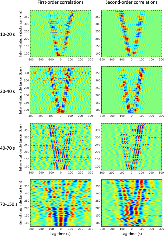
2.2. Bayesian and transdimensional inference
A primary objective of (isotropic) seismic tomography of the Alpine lithosphere is a depth map of the crust-mantle boundary at a resolution of a few tens of km. More precisely, a geological [Calcagno et al. 2008] and potentially geodynamic modeling of the mountain belt requires depth maps of the superposed European, Adriatic and Ligurian Moho surfaces affected by the subduction of the Alpine Tethys, the following collision of the European and Adriatic margins, and the opening of the Ligurian backarc basin. Seismic studies prior to the AlpArray project mapped the European Moho to a maximum depth of 55 km below the belt axis [e.g., Spada et al. 2013; Stehly et al. 2009; Kästle et al. 2018]. Receiver functions of the CIFALPS transect in the south-western Alps provided the first seismic evidence for continental subduction, including converted waves on the deep European Moho at 75–80 km beneath the westernmost Po plain, and negative-polarity conversions on an “inverted” Moho between the Adriatic mantle wedge on top and the European crust below, as shown in Figure 3b [Zhao et al. 2015; Paul et al. 2022].
Cross-sections along the CIFALPS profile in the southwestern Alps (CC′, location shown in Figure 1b). (a) Bouguer anomaly from Zahorec et al. [2021]; IGA: Ivrea gravity anomaly. (b) Common-conversion point (CCP) stack of receiver functions at stations of the CIFALPS experiment; locations of stations projected onto the CIFALPS profile are shown as black inverted triangles at the surface; the solid thick black lines are the European Moho (EurM) and the Adriatic Moho (AdM) that appear as converted waves of positive amplitude (in orange-red); the dotted thick black line shows an inverted Moho (InvM, higher velocity on top than on the bottom), which is marked by converted waves of negative amplitude (in blue); modified from Paul et al. [2022]. (c) Shear-wave velocity model from the ambient noise tomography of Lu et al. [2018]. (d) Shear-wave velocity model from the ANT with transdimensional inversion to Vs by Zhao et al. [2020]. (e) Shear-wave velocity model from the ambient noise tomography of Nouibat et al. [2022a]; dashed black line: Vs = 3.8 km/s velocity contour; continuous black line: Vs = 4.3 km/s velocity contour (Moho proxy); the thick grey lines are the Moho boundaries shown as black lines in (b). (f) Shear-wave velocity model from the ambient noise wave-equation tomography of Nouibat et al. [2023].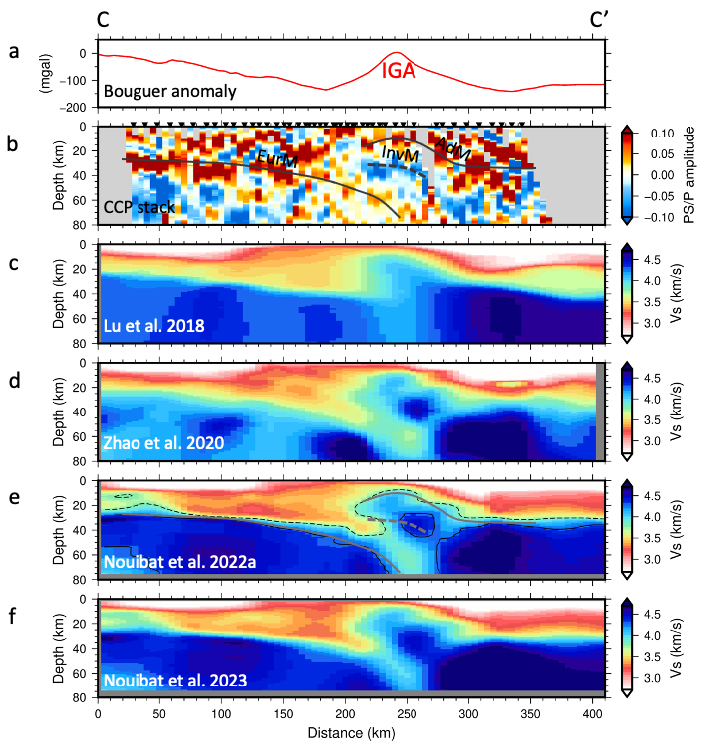
To take full advantage of the increased station density and to avoid dependence on arbitrary choices such as an initial model, several improvements were made to the inversions for Vs with depth.
2.2.1. 1-D depth inversion for Vs with a full exploration of the model space
A first improvement of the 1-D inversion for Vs was performed by Lu et al. [2018], who used a subset of AlpArray data, as station installation was still ongoing. Their inversion for group velocity maps involved a linearized inversion method based on ray theory [Boschi and Dziewonski 1999], and an adaptive parameterization scheme that reduced cell size in areas with high path density.
In the 1-D inversion stage for Vs, they built upon the inversion method of Macquet et al. [2014], where a full exploration of the model space was combined with a linear inversion for Vs. In this way, Lu et al. [2018]’s inversion for Vs included two steps. The first one used a grid search approach to uniformly sample and calculate group velocity dispersion curves for a low-dimensional model space based on a three-layer crust above a mantle half-space. This full model exploration was feasible because the dispersion curves can be computed with normal mode summation, and is computationally tractable. It was thus possible to determine an ensemble of models for which the dispersion curve matched the observed one. This first inversion step provided for each geographical grid cell a probabilistic Vs model and the probability to have a layer boundary at a given depth. However, to reduce the size of the model space to explore, the parameterization did not allow for low velocity zones. The second step was a linear inversion for Vs, where the problem was linearized around the mean of the probability distribution obtained at the previous step.
The dense station coverage and the two-step 1-D inversion scheme for Vs combining probabilistic sampling and linear inversion resulted in a (pseudo) 3-D Vs model with significantly higher spatial resolution than, for example, the model by Kästle et al. [2018]. Comparison with controlled-source reflection profiles [ECORS-CROP: Sénéchal and Thouvenot 1991; TRANSALP: Kummerow et al. 2004] and receiver function stacked sections across the Alpine belt [TRANSALP: Kummerow et al. 2004; CIFALPS: Zhao et al. 2015; Paul et al. 2022] displayed striking coincidence in Moho depth despite the poor sensitivity of surface-wave dispersion to layer boundaries (see Figures 3b,c for the CIFALPS transect). Lu et al. [2018] computed three depth maps of Moho proxies in the Alpine region using the probability of interface occurrence, the depth gradient of Vs and the isovelocity surface Vs = 4.2 km/s. These maps revealed new features such as an 8-km abrupt Moho step beneath the external crystalline massifs of the Western Alps, from Pelvoux to Mont-Blanc, which had not been detected by the ECORS-CROP DSS profile presumably due to poor signal penetration.
The 3-D Vs model by Lu et al. [2018] however failed to clearly image the continental subduction of Europe beneath Adria in the western Alps, which had been identified by receiver functions (Figures 3b,c). Since the inversion of Lu et al. [2018] was based on a simplified parameterization (only three crustal layers), and on a final optimization framework, the solution was a unique model that explains observations, but without associated uncertainties and trade-offs. In this way, this unique solution did not depict the full state of information contained in the data.
2.2.2. 1-D depth inversion for Vs with transdimensional inference
The next step in methodological improvement was therefore to carry out inversions within a full Bayesian framework and a fully adaptive parameterization, without any linearization, and where the solution is a full probability distribution, therefore providing uncertainty estimates. In this context, Zhao et al. [2020] performed a Bayesian transdimensional inversion of the group-velocity Rayleigh-wave dispersion data of Lu et al. [2018] with a focus on the western Alps (4.5°E–9°E; 44°N–46.7°N). Unlike the inversion by Lu et al. [2018], which assumed a four-layer model, the transdimensional inversion treats the number of layers as an unknown parameter [Bodin et al. 2012; Yuan and Bodin 2018]. At each gridpoint, Zhao et al. [2020] inverted dispersion data for Vs perturbations around a homogeneous half-space reference model with velocity 3.8 km/s, allowing a wide range of velocity variations (±50%).
The resulting (pseudo) 3-D Vs model (Figure 3d) displays a channel of anomalously low shear-wave velocities (Vs = 3.6 km/s) at 70-km depth beneath the fast-velocity, high-density Ivrea body anomaly in the CIFALPS cross-section (IGA in Figure 3a). This low-velocity anomaly is located between the deep European Moho and the inverted Moho of the Ivrea body imaged by receiver functions of the CIFALPS experiment (Figure 3b). The transdimensional inversion of Zhao et al. [2020] was thus able to image the subduction of the European continental lithosphere beneath the Adriatic lithosphere with minimal a priori constraints.
2.2.3. 3-D tomography with transdimensional inversions
The third methodological improvement carried out by Nouibat et al. [2022a] was to use the entire AASN dataset and apply a full transdimensional approach at both stages of the inversion, that is in the 2-D inversions for group velocity maps and in the 1-D inversions for Vs. At each period, a transdimensional inversion was carried out to obtain probabilistic Rayleigh-wave group-velocity maps following Bodin et al. [2012]. In the second stage, a full transdimensional approach was used to invert for Vs at each geographical location the dispersion curve obtained in the first stage.
The key benefit of the transdimensional inversion for group velocity maps is that spatial parameterization is treated as part of the inversion, allowing local resolution to adapt to data density. Another improvement introduced by Nouibat et al. [2022a] is the computation of uncertainties on group velocity estimates by transdimensional inversion; these uncertainties are then incorporated into the inversion for Vs (second stage). Young et al. [2013] and Pilia et al. [2015] were the first studies to use this two-step transdimensional procedure, with uncertainty computed in the first stage used to weight the input in the second.
In the first stage, to account for the strong lateral velocity contrasts of the Alpine crust, straight rays of the classical forward model were replaced by bent rays with the ray geometry updated at each iteration using the fast marching method of Rawlinson and Sambridge [2004]. Nouibat et al. [2022a] applied this new inversion scheme to four years of noise records from ∼1440 permanent and temporary seismic stations, including the entire AlpArray network with its offshore component (Z3 network: AlpArray Seismic Network 2015), the two CIFALPS experiments [YP and XT networks: Zhao et al. 2016b, 2018], and the EASI experiment [XT network: AlpArray Seismic Network 2014] (Figure 1). Data coverage is improved compared to Lu et al. [2018], and so to Zhao et al. [2020], especially in the Western Alps and the Ligurian Basin.
Figure 3e shows a depth section along the CIFALPS transect in the 3-D Vs model by Nouibat et al. [2022a], which may be compared to the models by Lu et al. [2018] shown in Figure 3c, and Zhao et al. [2020] shown in Figure 3d. Unlike Lu et al. [2018] and similar to Zhao et al. [2020], Nouibat et al. [2022a] image the dipping low-velocity layer beneath the Ivrea body high-density, high-velocity anomaly (IGA, x = 210–300 km in Figure 3), which is indicative of the continental subduction of Europe beneath Adria. As the Zhao et al. [2020] inversion for Vs was based on the same dispersion dataset as Lu et al. [2018], and as Nouibat et al. [2022a] used the same inversion method for Vs as Lu et al. [2018], but with a different set of four-layer models, we propose that the major difference between Figures 3c and 3e is related to the difference between the sets of velocity models explored in the probabilistic inversion for Vs: 130 million for Nouibat et al. [2022a], and 8 million for Lu et al. [2018]. In particular, the complex vertical velocity profiles of the subduction region with alternating high and low velocities were not explored by Lu et al. [2018]. Vertical velocity gradients are stronger in Nouibat et al. [2022a]’s model (Figure 3e) than in Zhao et al. [2020]’s model (Figure 3d), in particular at the crust-mantle boundary. Even though the input data and the inversion schemes differ, the overall similarities between the two models of Figures 3e and 3f suggest that the differences in velocity gradient at the Moho may result from the parameterization of the inversions for Vs. While the probabilistic inversion of Nouibat et al. [2022a] assumes a four-layer starting model with a velocity jump at Moho, the reference velocity model in the transdimensional inversion of Zhao et al. [2020] is a homogeneous half-space with no discontinuity. This a priori uniform distribution of velocity may favor a smooth velocity gradient at Moho. The Vs model by Nouibat et al. [2022a] with its a priori imposed sharp crust-to-mantle velocity contrast is more in line with previous controlled-source (ECORS-CROP in the north-western Alps) and receiver function profiles [CIFALPS: Figure 3b; CIFALPS-2, Paul et al. 2022], which display clear reflected and converted phases on the Moho. The impact of other refinements in the Nouibat et al. [2022a] inversion methodology (error estimates on group velocities, bent rays) is difficult to evaluate due to the differences in the input data coverage. It would be an interesting test to apply the fully transdimensional inversion for Vs of Zhao et al. [2020], with an a priori constraint on the velocity jump at the Moho, to the group velocity data with uncertainties of Nouibat et al. [2022a].
2.3. Wave-equation tomography
To compute shear-wave velocity models of the crust and uppermost mantle from Rayleigh-wave traveltime data between station pairs, Lu et al. [2018] and Nouibat et al. [2022a] have used a two-stage inversion scheme, which, in spite of improvements related to a probabilistic approach, is a standard strategy for ANT. The first stage, a series of 2-D inversions of traveltime data for group velocity maps at selected periods, is based on ray theory, which is only valid at infinite frequency. The second stage, a set of 1-D inversions of the local dispersion curves for S-wave velocity, results in 1-D models merged into a pseudo 3-D model. The strong crustal heterogeneity of the Alps and surrounding areas, including the Ligurian back-arc basin, makes the ray hypothesis particularly inadequate. This area therefore provides an excellent chance of testing a tomography procedure that better accounts for the physics of seismic wave propagation. In this section, we first describe a new wave-equation based approach of ambient noise tomography called wave equation tomography [WET, Lu et al. 2020] for the elastic case, using only land station recordings. We next present the extension of the WET method to include elastic–acoustic coupling at the sea bottom and OBS records [Nouibat et al. 2023].
2.3.1. Wave-equation onshore tomography (elastic case)
To calculate a truly three-dimensional Vs model consistent with wave propagation physics, Lu et al. [2020] derived a wave-equation based approach, hence called ambient noise wave-equation tomography. As in the ambient noise adjoint tomography of Chen et al. [2014], the observable is travel time (i.e. phase) of the Rayleigh wave reconstructed from noise correlation, while full-waveform inversion (FWI) would invert amplitude and time. Indeed, Rayleigh wave amplitudes are not correctly retrieved by the classical noise correlation procedure [e.g., Campillo 2006]. FWI of ambient noise correlation signals probably has great potential for lithospheric imaging. It is not yet operational because it would require specific pre-processing of noise records for a better retrieval of amplitudes and, more importantly, an accurate estimate of noise source distributions and emitted waveforms [e.g., Fichtner 2014; Sager et al. 2018].
The wave-equation tomography (WET) approach implemented by Lu et al. [2020] consists of iteratively updating an initial ambient noise tomography model (from the two-stage traditional method) by minimising frequency-dependent phase traveltime differences between the Rayleigh waveforms observed in noise correlations and the synthetic waveforms computed by 3-D numerical modeling of wave propagation. Synthetic waveforms are computed with the 3-D elastic wave equation solver of the SEM46 package [Trinh et al. 2019] based on the spectral element method [Komatitsch and Vilotte 1998; Komatitsch and Tromp 1999]. Of the 304 stations located in the study region, a subset of 64 suitably located stations were selected as virtual sources by Lu et al. [2020], and the signal bandwidth was limited to [10–50 s] to ensure acceptable computing time. The observed signal for a station pair is the Rayleigh wave part of the Green’s function, estimated from the time derivative of the cross-correlation of seismic noise. The synthetic signal is the convolution product of a bandpass filtered Dirac delta source function with the synthetic Green’s function computed with SEM46 for a source–receiver pair, and a vertical force applied on the free surface at the source location. The misfit function is then computed from the frequency-dependent phase traveltime differences between observed and synthetic waveforms. The adjoint-state approach is used to compute the misfit gradients [e.g., Tromp et al. 2005], and the inversion is conducted as an iterative local optimization problem.
The final S-wave velocity model obtained by Lu et al. [2020] after 15 iterations of wave equation tomography has a 65% lower total misfit than the initial ANT model by Lu et al. [2018]. This strong misfit reduction is mostly due to periods larger than 25 s, where the WET has corrected for a strong and unexplained positive shift of the traveltime misfit histograms in the initial model. A direct consequence is that the final Vs model has significantly higher average velocities at lower crustal depth (30 km). Beyond this tuning of average velocities, the WET approach was able to retrieve finer scale heterogeneities than the ANT model, for example a high-velocity anomaly at 10 km depth, which is closer in shape to the well-known Ivrea positive Bouguer anomaly [see Figure 8 in Lu et al. 2020].
2.3.2. Wave-equation onshore/offshore tomography (with acoustic–elastic coupling)
As compared to Lu et al. [2018], a more accurate ANT model of the Alpine region and its surroundings was computed by Nouibat et al. [2022a] using a larger noise correlation dataset including recordings of sea-bottom seismometers in the Ligurian basin, and an improved inversion scheme (see Section 2.2). Like Lu et al. [2020], Nouibat et al. [2023] have performed a WET to improve the model of Nouibat et al. [2022a] by accounting for three-dimensional and finite-frequency effects of wave propagation. A major improvement achieved by Nouibat et al. [2023] is the inclusion of the water layer effect on wave propagation in the Ligurian basin. The vertical-component record of short-period (<20 s) surface waves at ocean-bottom stations is dominated by a fluid–solid interface wave named Rayleigh–Scholte wave that propagates at lower speed than the Rayleigh wave in the elastic medium. At periods >20 s, the effect of the water layer becomes negligible for the Ligurian basin (max. water depth 3 km) because the Rayleigh wavelength is large compared to water depth [Nouibat et al. 2023]. Accounting for the effect of the water layer in the forward simulation of surface-wave propagation and in the inversion of traveltime observations for shear-wave velocity is therefore required to enhance resolution in the shallow layers of the Ligurian basin.
For their wave-equation tomography with elastic–acoustic coupling, Nouibat et al. [2023] selected, from the dataset of Nouibat et al. [2022a], 600 stations as receivers, out of which 185 were selected as sources based on noise correlation signal quality. The initial model was the ANT Vs model computed by Nouibat et al. [2022a]. As in Lu et al. [2020], the inverse problem minimised the frequency-dependent phase traveltime differences between observed and synthetic vertical-component waveforms for considered source–receiver pairs. The inversion was conducted in the 5–85 s period range, considering elastic–acoustic coupling in the forward simulation in the 5–20 s band. Unlike Lu et al. [2020], the velocity model was updated progressively from long periods (40–85 s) to shorter ones, 20–40 s, 10–20 s then 5–10 s to avoid cycle skipping.
The final WET Vs model differs significantly from the initial ANT Vs model, particularly in shallow layers of the Ligurian Basin, and in the most heterogeneous parts of the Alpine crust. These discrepancies highlight the importance of accounting for the physics of wave propagation, i.e. elastic–acoustic coupling at the sea-bottom, finite-frequency effects and 3-D propagation. In the alpine crust (i.e. onland), velocity contrasts tend to be slightly enhanced, in particular at lower crustal depth [26 km, see Figure 6 in Nouibat et al. 2023], while the location and shape of velocity changes are preserved with respect to the initial ANT model (Figures 3e–f). At depths shallower than ∼10 km, S-wave velocities in the Ligurian basin are ∼8% lower in the WET model than in the ANT model, in agreement with the lower velocities of the Rayleigh–Scholte wave. Accounting for the water layer in the Ligurian basin also leads to higher velocities in the crust of western (Variscan) Corsica.
Nouibat et al. [2023] conducted extensive evaluation of the robustness of their WET model. The quality of the S-wave velocity model was documented by traveltime misfit maps at representative periods between 8 and 55 s. As expected, misfit is lower for the WET model than for the initial ANT model, except in the peripheral poorly illuminated regions [see Figure 12 in Nouibat et al. 2023]. The footprint of the broad geological structure has disappeared, whereas it was clearly visible for the ANT model at periods ⩾20 s. Using the weak sensitivity of Rayleigh wave phase velocity to Vp, Nouibat et al. [2023] also inverted Rayleigh wave dispersion observations for P-wave velocity, starting from an initial Vp model computed from the initial (ANT) Vs model using an empirical formula. To document the robustness of their P and S-wave models, they computed synthetic waveforms for a regional earthquake in Switzerland and compared to observed waveforms in three frequency bands between 2 and 10 s. The fit between simulated and observed seismograms is striking for the travel times of the P and Rayleigh waves, but also for relative amplitudes between the wave trains. Such a high coherence in the short-period bands is a reliable indication that wave equation tomography is capable of imaging small-scale crustal structures. This synthetic test also demonstrates that the WET Vs and Vp models derived from ambient noise correlations would be a good initial model for a wave-equation tomography using earthquake records. As regional earthquake records include both body and surface waves, the resulting P-wave velocity model would be much more accurate than that obtained from Rayleigh wave travel time inversion alone, due to its weak sensitivity to Vp.
2.4. Model validation: Moho depth
Surface waves are weakly sensitive to velocity contrasts, but Bayesian inversions for Vs were shown to be very effective for imaging the crust-mantle boundary [Lu et al. 2018; Nouibat et al. 2022a]. Comparisons of Moho depths imaged by other geophysical methods such as DSS profiles (ECORS-CROP) and receiver function analyses have shown that selected iso-velocity surfaces in the ambient noise derived 3-D Vs models are reliable proxies of the Moho [Nouibat et al. 2022a; Paul et al. 2022; Nouibat et al. 2023]. For example, the velocity contour Vs = 4.3 km/s is a good proxy for the European Moho, and the Adriatic Moho outside the Ivrea body region, as shown by the coincidence of this surface with Moho conversions picked from CCP receiver function stacks along the CIFALPS and CIFALPS2 sections (see for example Figure 3e). In the Ivrea body region, the Moho imaged by the ECORS-CROP DSS profile and receiver function sections is better approximated by the 3.8 km/s velocity surface, probably because the external rim of the Ivrea body is made of serpentinized peridotites with lower velocities than dry peridotites [Figure 3e; see discussion in Malusà et al. 2021]. In the Ligurian basin, a comparison of the Vs model of Nouibat et al. [2022a] with a Vp model derived by Dannowski et al. [2020] from refraction and wide-angle reflection OBS data shows a striking coincidence of the Vp Moho (iso-velocity 7.2 km/s) with the 4.1 km/s Vs contour [see Figure 9 in Nouibat et al. 2022b]. A Moho depth map of much higher resolution than previous ones [e.g., Grad et al. 2009; Spada et al. 2013] can therefore be built by mapping iso-velocity contours of the Vs models by Nouibat et al. [2022a] and Nouibat et al. [2023].
3. Anisotropic ambient noise tomography
Surface waves in seismic noise correlations can potentially shed new light on anisotropy in the Earth’s crust and upper mantle, overcoming the observational biases related to the uneven distribution of earthquakes, which leads to uneven azimuthal coverage [for a review, see Maupin and Park 2015].
Our knowledge of azimuthal anisotropy beneath the Alps and Italy mostly comes from XKS splitting studies. Fast velocity directions are generally parallel to the mountain chain in the Western and Central Alps [Barruol et al. 2004, 2011; Lucente et al. 2006; Salimbeni et al. 2018], the Eastern Alps [Bokelmann et al. 2013; Qorbani et al. 2015] and the Apennines [Palano 2015]. Teleseismic P wave travel time delays were used by Rappisi et al. [2022] to study anisotropy in the Central Mediterranean area, including the Alps. Both XKS and teleseismic P waves have too steep incidence angles to reliably constrain anisotropy in the crust, also because the cumulated travel time in the crust is much smaller than in the upper mantle. Studies using regional refracted Pn and Sn phases like Díaz et al. [2013] provide information about the uppermost mantle, as these waves are tied to the Moho interface and propagate with mantle velocities.
Long wavelength anisotropic structure beneath Europe is mostly known from large scale or global surface wave studies where the crust is not resolved [e.g., Kustowski et al. 2008; Weidle and Maupin 2008; Boschi et al. 2009; Zhu et al. 2015; Nita et al. 2016; Schivardi and Morelli 2011]. All these studies are constructed from long period observations, where the crust is not inverted for but set from a reference model such as LITHO1.0 [Pasyanos et al. 2014]. A few studies focussing on crustal anisotropy used surface waves from seismic noise correlations to characterise anisotropy at regional scale, such as Switzerland [Fry et al. 2010], the Vienna Basin [Schippkus et al. 2020], the Bohemian Massif [Kvapil et al. 2021], or the Eastern Alps [Kästle et al. 2024].
The dense station coverage (Figure 1) across the greater Alpine region during the AlpArray project provided a unique opportunity to further develop and understand the limitations of noise-based imaging methods aimed at characterising seismic anisotropy across a strongly heterogeneous structure. Since the Alpine region is heterogeneous at all scales, it is in particular crucial to reliably estimate uncertainties and identify locations and periods where systematic errors may affect azimuthal anisotropy measurements. These questions are the focus of Section 3.1.
Once uncertainties associated with surface wave velocities are estimated, they can be used in inversions for depth variations of anisotropic parameters. Reliable uncertainties are also crucial in the case of joint inversions, where different datasets are inverted simultaneously (e.g., earthquake based and noise-based observations). A Bayesian inversion framework in theory handles this question in a both intuitive and simple way, producing families of acceptable Earth models, over which it is possible to make posterior statistics. This ensemble solution can be exploited to give reliable and useful information on the Earth structure. Section 3.2 is dedicated to such strategies for both radial and azimuthal anisotropy.
3.1. Improving observations of azimuthal anisotropy
The effect of isotropic heterogeneities on the wavefield can map into anisotropic parameters. In this section, we give some insights into such effects through the now well-established Eikonal tomography method [Lin et al. 2009]. We present outcomes of Eikonal tomography across the Alps and show how beamforming can improve seismic noise-based observations of anisotropy. Both Eikonal tomography and beamforming naturally correct for deviations from great circle [e.g., Pedersen et al. 2015] and uneven distribution of noise sources [e.g., Froment et al. 2010; Harmon et al. 2010], so the only main bias to handle is the one from isotropic heterogeneities.
3.1.1. Biases in measurements of azimuthal anisotropy: insights from Eikonal tomography
Eikonal tomography makes use of dense station networks to reconstruct the wavefield propagating away from a source [Lin et al. 2009]. In ambient noise applications, any seismic station can act as a virtual source and the signals recorded at all other stations allow us to image the wavefield. When computing ambient noise correlations, amplitudes are lost due to filters such as spectral whitening. Only the travel-time field is recovered, therefore hindering the use of amplitudes to correct for bias from wave interference.
In Eikonal tomography [Lin et al. 2009], travel times recorded at receivers are interpolated onto a regular grid. The gradient of the travel-time field then gives the phase velocity and the propagation direction at each grid point. This highlights important strengths of Eikonal tomography: it is simple to calculate and the direction of the incoming wave is directly determined from the data. In order to get the full, azimuthal anisotropic phase velocity map, the process has to be repeated for all available virtual sources so that a set of phase velocity measurements and their propagation azimuths is obtained for each grid cell. The final phase-velocity field is obtained by averaging the measured phase velocities for all virtual sources. Different statistics of the estimated phase velocities (mean, median, mode and standard deviation) can be used as uncertainty estimates. Similarly, for the anisotropic part, the residual from the fitted function provides information on the reliability of parameter estimates.
Isotropic bias can be approximately modelled by a 360° variation of phase velocity with azimuth [Lin and Ritzwoller 2011; Mauerberger et al. 2021]. We refer to phase velocity variations with azimuth in the following form (applicable to weakly anisotropic media):
| (1) |
Figure 4 shows systematic errors resulting from isotropic heterogeneities through synthetic data computed in a laterally heterogeneous model, onto which we apply Eikonal tomography. In Figure 4d (perfect sampling), we observe an undulating pattern in the isotropic velocities, which depends on the signal wavelength. This undulating pattern is due to the interference of waves that are refracted by the isotropic anomaly. Most of the bias, however, cancels out when averaging over sources from many directions (Figure 4e). This error can also be corrected when taking the amplitude information into account [e.g., Helmholtz tomography, Lin and Ritzwoller 2011]. A more severe bias stems from under-sampling the wavefield (Figure 4b). To work properly, the Eikonal method requires approximately plane wavefront between adjacent receivers. If the medium is highly heterogeneous, this assumption is violated and only a smoothed version of the true wavefield can be reconstructed from the measurements at the receiver locations. The resulting error in the isotropic part mostly cancels out when signals from different azimuths are averaged (Figure 4c). In the anisotropic part, however, a systematic, azimuth-dependent error remains, resulting in spurious anisotropy around the edges of strong velocity heterogeneities.
Example illustrating the bias in the anisotropic Eikonal tomography method. (a) 2-D wavefield propagating away from the virtual source station; black dashed lines indicate the locations of isotropic high and low velocity anomalies. (b) Isotropic phase velocities recovered by applying the Eikonal tomography method to the wavefield recorded at the receiver locations; anomalies outside the dashed lines are mainly caused by incomplete reconstruction of the true traveltime field. (d) Same as (b) for a perfectly sampled traveltime field; the striped velocity heterogeneities behind the anomalies are caused by wavelength-dependent wave interference effects. (c) and (e) Final models resulting from averaging the models for all virtual sources, i.e., swapping the position of the virtual source with all available receiver positions. The apparent anisotropy (yellow bars) is caused by velocity errors illustrated in (b) and (d) since the input model is purely isotropic.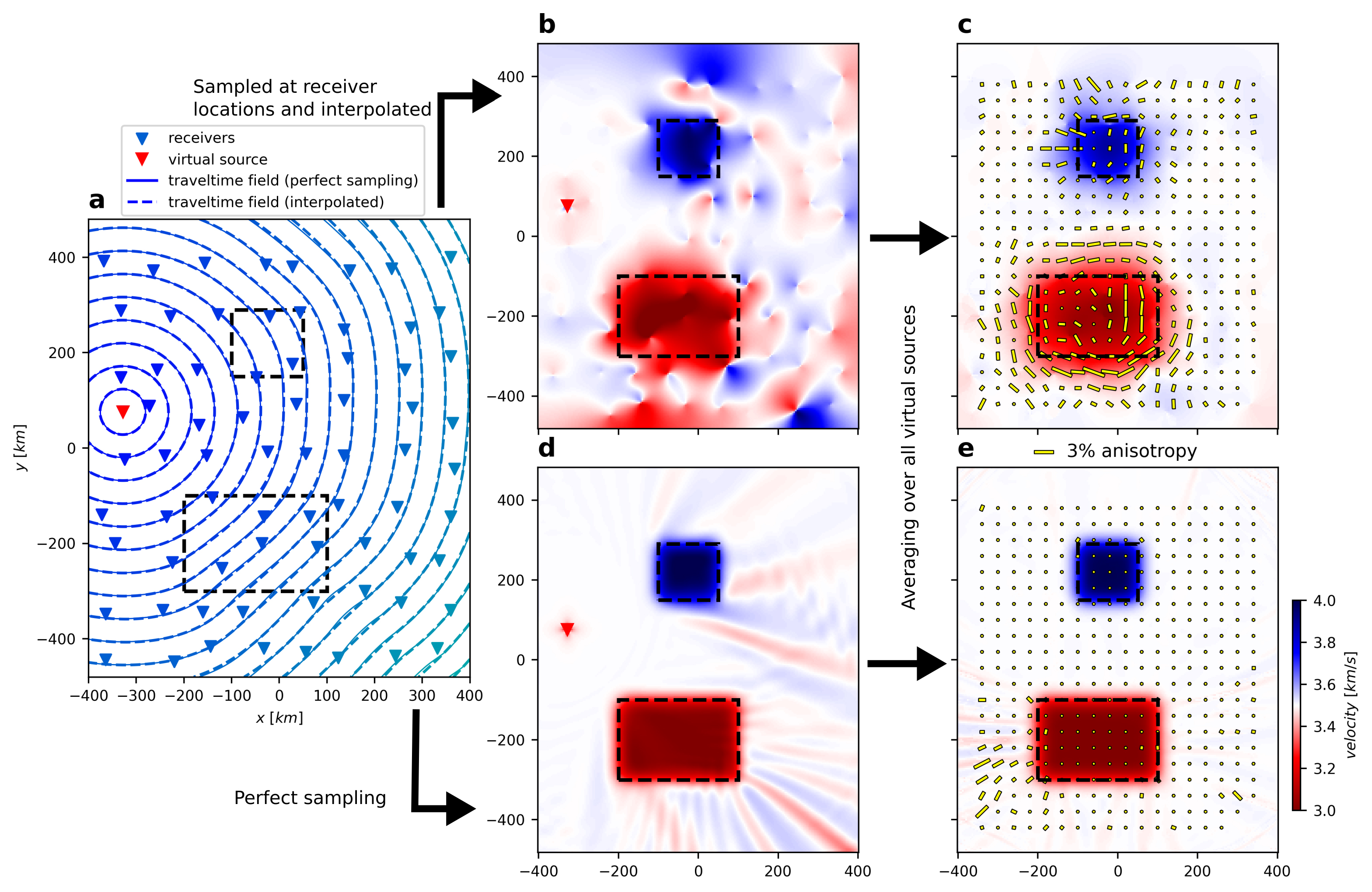
The level of these spurious anisotropic measurements depends not only on the absolute velocity variation but also on the wavelength of the signal, the inter-station spacing and the velocity gradient at the edges of the anomalies. The controlling factor for the bias is the level of complexity of the wavefront between adjacent stations.
3.1.2. Eikonal tomography in the Alps
Kästle et al. [2022] presented an application of Eikonal tomography to the Alpine area, including data from the AlpArray network. They were able to resolve both the isotropic and the anisotropic parts at periods sensitive to different depth ranges from the shallow crust to the uppermost mantle. The three anisotropic components were obtained by taking the azimuthally dependent phase-velocity measurements and fitting them to Equation (1).
Kästle et al. [2022] tested for different observables that can be related to a bias in anisotropy measurements, such as the amplitude of the 𝜃1 component or the standard deviation from fitting the 𝜃2 anisotropy. They found that none of these observations are adequate to reliably identify biased measurements. More sophisticated approaches such as forward modelling the travel-time field from the isotropic velocities may be necessary. This could also be used iteratively to improve the accuracy of the interpolation for highly complex travel-time fields, at the cost of giving up the relative simplicity of the Eikonal approach. However, Kästle et al. [2022] inferred from synthetic tests that isotropic anomalies of up to 10% produce bias, which in most cases is smaller than what is identified as “true” anisotropy.
The 𝜃2 anisotropic component obtained by Kästle et al. [2022] is presented in Figure 5. The fast axis directions generally follow the curvature of the Alpine arc at 15 s period, representative of the upper crust. At 40 s period, the fast axis becomes more oblique to orogen-perpendicular within the central Alps. The eastern part of the Alps has more homogeneously E–W oriented fast axes from short to long period measurements. In most of the northern Alpine foreland, the anisotropic fast axis orientations are consistently following the Alpine curvature at periods between 10 and 50 s.
Maps of 𝜃2 azimuthal anisotropy at 15 and 40 s period resulting from Eikonal tomography in the Alps. The direction of each line shows the fast direction, and the length shows the amplitude (zero to peak). The colour of the lines gives the estimated uncertainty on the amplitude A2 (in percent of C0).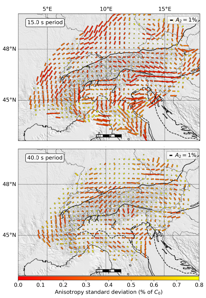
The uncertainties in the anisotropic measurements are largest at model boundaries, where the azimuthal coverage is non-optimal, as well as within and around the large sedimentary Po and Molasse basins north and south of the Alps. In the former, isotropic velocities indicate that velocities can be as low as −30% compared to the average velocity [Kästle et al. 2022]. These regions are therefore prone to the systematic bias mentioned above, particularly at short periods. In most of the other regions and at longer periods, the anomaly strength is usually within ±10% with smoothly varying isotropic velocities. Correspondingly, Kästle et al. [2022] found that the imaged pattern of anisotropies in the Alps is compatible with previous, more localised studies Fry et al. [2010], but also with the results from beamforming [Soergel et al. 2023; Section 3.1.3].
3.1.3. Beamforming
An alternative approach to Eikonal tomography is to use the phase information in a beamforming approach. Beamforming consists of, for a set of closely located seismic stations and at a given frequency, inferring the direction and local phase velocity of the incoming wave [for a review, see Rost and Thomas 2002]. Contrary to Eikonal tomography, the full waveform of the empirical Green function is used, as illustrated in Figure 6. The original waveforms (Figure 6a) are shifted in time using a grid search across many phase velocities and incoming directions. The final estimated phase velocity is the one for which the traces are optimally aligned (Figure 6b), and for which the stack yields the highest maximum amplitude (Figure 6c).
Illustration of data processing, and map of estimated azimuthal anisotropy at 15 s period for one seismic array. (a) Filtered traces before aligning. (b) Same traces as (a), aligned using the combination of azimuth and phase velocity for which the stack is optimal (maximum peak amplitude). (c) Stack at optimal parameters, normalised by the number of stations. The maximum of this stack is called dmax. (d) Phase velocity as a function of azimuth, using all source stations. The orange and green curves correspond to the first two cosine terms of Equation (1). (e) Number of source stations (binned in 5° azimuth bins) as a function of azimuth. (f) Quality of stack dmax for all source stations. The seismic array is centered at the blue dot. It is surrounded by a blank area, because of the need to respect a minimum distance between source and receiver stations. The colour code shows dmax, the maximum amplitude of the stack divided by the number of traces. Soergel et al. [2023] particularly focused on quality control and error estimates to be able to carry out inversions for anisotropic parameters with depth. Such quality control and error estimates are key input for subsequent transdimensional Bayesian inversion described in Section 3.2.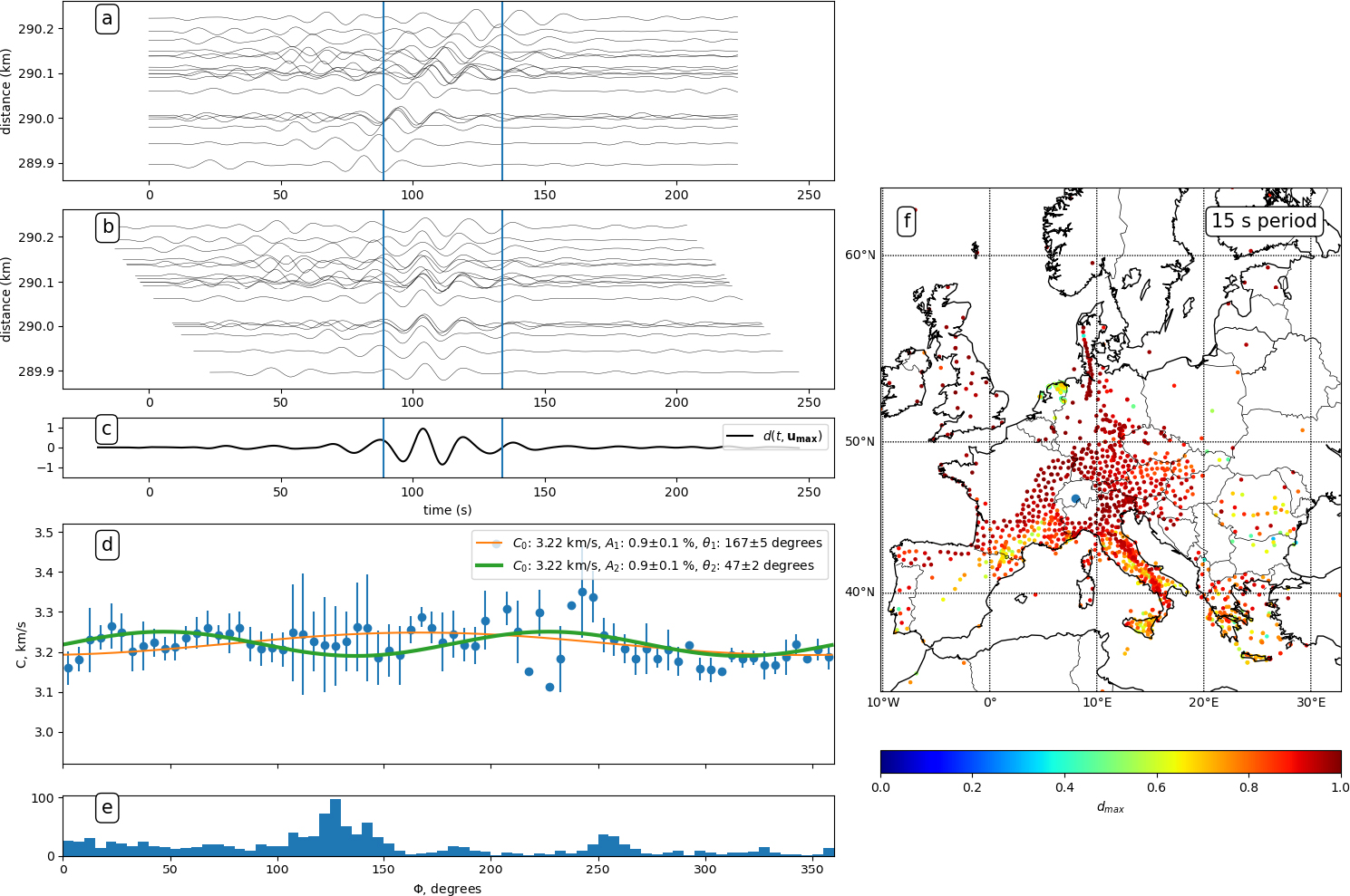
Beamforming has been extensively used on seismic noise, in particular to characterise the noise field and infer the locations of origin of noise sources [for Europe, see for example Friedrich et al. 1998; Landès et al. 2010 or Juretzek and Hadziioannou 2016]. Beamforming has also been used to quantify anisotropy on earthquake data [e.g., Pedersen et al. 2006; Alvizuri and Tanimoto 2011] or directly on raw noise records [e.g., Riahi and Saenger 2014].
To estimate surface wave azimuthal anisotropy, beamforming has to be carried out, for each source, across the range of target periods (Figure 6d).
This method was previously used on earthquake data. Applying it to noise correlation is straightforward as seismic stations can be used as virtual sources. Here we present key elements of the implementation of Soergel et al. [2023] and the application to the Alps. A somewhat similar approach was taken at the same time by Wu et al. [2023] for the Northeastern Tibetan Plateau.
The specific choices made to adapt the beamforming included:
- Using seismic stations outside the study area as virtual sources, to improve azimuthal coverage at the edge of the study area.
- Taking into account the short distances between the array and the “source” station. This was done mainly by assuming circular wavefronts following Maupin [2011] rather than plane wavefronts, and imposing a minimum distance between array and “source” station. The implementation still allowed to take into account great-circle deviations, which can be significant across AlpArray.
- Propagating uncertainty of each data point (phase velocity at a given period for a given array and source stations, see example in Figure 6f). This is done by weighting each observed phase velocity for the estimate of the A2 and 𝜃2 terms for a given array at a given period, with the normalised beam amplitude dmax, and use of bootstrap to estimate the uncertainty on A2 and 𝜃2.
- Exclusion of data points if the isotropic bias (estimated by A1) is significant.
- Adapting array geometry to wavelength and noise levels.
Figure 7 shows two examples of surface wave azimuthal anisotropy measured with this method across the Alpine area, at 15 s and 40 s period. Points with risk of a strong isotropic bias (high value of A1 as compared to A2, see Equation (1)) are excluded from the maps. In many points, the bias was particularly strong at periods which are sensitive to changes in Moho depth, and was overall coherent with areas of strong isotropic velocity gradients. For further discussion, we refer to Soergel et al. [2023].
Maps of azimuthal anisotropy at 15 s and 40 s period resulting from the beamforming method. The direction of each line shows the fast direction, and the length shows the amplitude. The colour of the lines show the estimated uncertainty on the amplitude A2 (in percent of C0).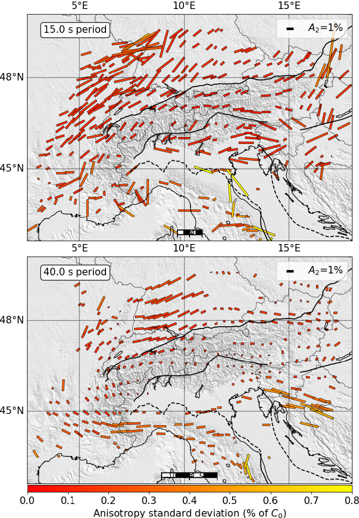
The beamforming yields spatially coherent patterns of azimuthal anisotropy across all of the study area. Overall, the beamforming is in good agreement with the Eikonal method (Figure 5) on key findings, such as (at 15 s period) lower amplitude anisotropy within the Alps as compared to surrounding areas, and the surrounding areas being dominated by chain parallel fast direction. There are main differences at the periphery of the study area, which can be explained by the lack of azimuthal coverage in the Eikonal tomography. Lateral smoothing effects are also different between the two methods. While the reliability of the beamforming is high due to the point by point (geographically, for each period) evaluation of quality and errors, it also leads to changing geographical distributions of reliable data with period, and the implementation would need to resolve this issue to be able to provide 3-D models of anisotropy.
Depth inversions for azimuthal anisotropy must be considered a priority in anisotropic studies because of the wide range of possible values of A2. For example, if the upper crust is strongly anisotropic and neither lower crust or upper mantle are anisotropic, the observed anisotropy at, for example, 40 s period still has its origin in the upper crust. Similarly, changes in fast direction in layers with small anisotropy are not directly visible at any given period. Whether small amplitude anisotropy is resolved therefore strongly depends on the observation error. The strong control of errors provided by beamforming is consequently key for the depth inversions which are addressed in the following section.
3.2. Transdimensional Bayesian inversions of anisotropic measurements
Similar to isotropic inversions, once surface wave velocities have been estimated at different periods, they can be inverted to recover anisotropic shear wave velocity structure at depth. This is usually done in a second inversion step carried out at each geographical location. Rayleigh and Love dispersion curves can be jointly inverted for radial anisotropy parameters with depth. In the case of azimuthal anisotropy, Rayleigh and Love wave dispersion curves and their azimuthal dependency at each period can each be inverted to obtain azimuthal anisotropy parameters with depth.
Fortunately, this inverse problem is only weakly nonlinear, and many linearized approaches have been used, where data derivatives (sensitivity kernels) computed around a reference model are used. However, the solution is highly non-unique, as surface waves are only sensitive to integrated velocities along a depth range. In the case where seismic anisotropy is inverted for, the non-uniqueness of the solution becomes particularly problematic as strong trade-offs emerge between different parameters. For example, the level of radial anisotropy trades off with Vp and with the level of heterogeneities in Vs [Bodin et al. 2015; Alder et al. 2017; Gao and Lekić 2018], because of the equivalence of a stack of horizontal layers and a homogeneous anisotropic medium [Backus 1962].
To add extra constraints on the solution, some regularisation can be used at the cost of biasing estimated uncertainties in the recovered model. In this way, linearized approaches only provide a unique velocity model that does not represent the range of potential solutions, and that is strongly dependent on the regularisation, the parameterization, or the reference model. For example, the Vp model is often set to a reference or arbitrarily scaled to Vs variations. The level of smoothness is also set in advance. Although these choices are based on geological or mineralogical arguments, they make the interpretation of results dependent on a priori choices.
Similar to isotropic inversions, these issues can be addressed by fully exploring the range of potential solutions with Monte Carlo methods (see Section 2.2.1). Since forward simulations are computationally cheap, a large number of 1-D models with variable parameterizations can be tested to sample complex posterior distributions. Adaptive parameterizations can be used to explore complex trade-offs between model parameters. For example, a transdimensional parameterization (where the number of model parameters is variable) can be used to explore the ambiguity between the level of spatial heterogeneity (horizontal layering) and the level of anisotropy created by the orientation of anisotropic minerals [Bodin et al. 2015, 2016; Alder et al. 2017]. In this case, the total number of layers in the inverted model as well as the presence of anisotropy in each layer are not constant parameters. Instead, they are adjusted by the inversion to fit the data to the degree required by their estimated noise. In this context, the Bayesian framework enables to propagate estimated uncertainties in the observed dispersion curves towards uncertainties in shear wave velocities at depth.
3.2.1. Adaptive parameterizations: example with radial anisotropy
To illustrate the benefit of such flexible parameterizations, we first show in Figure 8 an example of a synthetic test taken from Alder et al. [2021]. A target model is designed with a radially anisotropic layer in the crust and an isotropic upper crust and mantle. Noisy synthetic data are created and inverted with a transdimensional Monte Carlo algorithm, but with two different types of parameterizations (left and right panels). On the left, the number of layers is variable and each layer can be either isotropic and described solely by Vs and Vp (in this case, radial anisotropy in the form VSH∕VSV takes a constant value of 1), or radially anisotropic and described by three parameters: VSV, Vp and the level of radial anisotropy VSH∕VSV. In this way, the number of inverted physical parameters in each layer is variable. On the right panel, the number of layers is also variable but all layers are radially anisotropic and described by three parameters. Everything else is equal in the two inversions.
Joint inversion of Love and Rayleigh wave synthetic dispersion curves. The same data produced by the true model are inverted with two different procedures. Posterior distributions of VSV (red), and VSH∕VSV (blue). The true model used to create synthetic data is the thick solid line in every panel and the mean of the prior distribution used in the inversion is the grey line in the VSV panel. Posterior distributions are depicted with their median (thin solid line) and likelihood intervals: for each parameter, the dark surface includes 65% of the models in the ensemble solution while the light area includes 95% of the models. Left panels: inversion used in Alder et al. [2021], where each layer can either be isotropic or anisotropic. Right panels: inversion where anisotropy is imposed as an unknown parameter at all depths. Modified from Alder et al. [2021].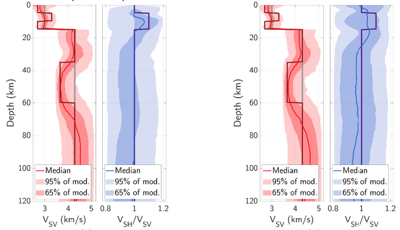
Although the shear wave velocity is equally well resolved in both cases, the anisotropic layer in the crust is better recovered with the flexible scheme on the left. In the mantle, where the true model is isotropic, the ensemble solution produced on the left panel includes a large number of isotropic models, resulting in a narrower distribution for radial anisotropy and a median value of the distribution equal to unity. Conversely, in the case where anisotropy is imposed at all depths (right panels), a wider distribution of anisotropy is obtained, resulting in wider uncertainties.
This comparison shows that in the case of a true isotropic model, a flexible parameterization allows fitting data with simpler isotropic models that are described by fewer parameters. The result of the inversion is a distribution of models which is closer to the true model.
3.2.2. Exploiting the full wealth of information in posterior distributions: example with azimuthal anisotropy
The previous example shows the benefits of using complex adaptive parameterizations in Bayesian inversions. The solution is not a single model, but an ensemble of models with variable parameterizations that approximates a probability distribution defined in a multiple dimensional space. As shown in Figure 8, one simple way to exploit this complex solution is to extract the mean or median value for a given parameter at each depth. Standard deviations can also be used, but more information is available about posterior covariances and trade-offs, and inference about these quantities can be hard to make. This wealth of information can be exploited through different angles of analysis and visualisation, each one giving additional insight to specific geophysical questions.
We illustrate this in Figure 9 where Rayleigh wave dispersion curves and their azimuthal variations measured from beamforming (see Section 3.1.3) are inverted at depth following the method of Bodin et al. [2016]. Here, the number of layers is variable and each layer is either isotropic and described solely by its isotropic shear-wave velocity, or azimuthally anisotropic and described by three parameters: (1) the isotropic shear-wave velocity; (2) the peak to peak level of azimuthal anisotropy, and (3) the direction of the horizontal fast axis relative to the north [Romanowicz and Yuan 2012].
Depth inversion of Rayleigh wave surface wave dispersion curves with azimuthal variations for a subarray located in the Dinarides. The solution is a large ensemble of models with different parameterizations (different numbers of isotropic and anisotropic layers). (a) Probability distribution of the amplitude. (b) Probability distribution of the direction of the fast axis of anisotropy. The black line in (a) shows the average amplitude, and the horizontal black lines in (a) and (b) indicate the limits of the three layers over which we integrate anisotropy. (c) Density plot of anisotropy parameters integrated over the three different depth ranges. The radius in the polar plots indicate amplitude and the angle gives direction of the fast axis of anisotropy. The colour scale indicates the normalised probability of a given combination of amplitude and fast direction. Panels (d) and (e) show the marginal distributions of 𝛿Vs (d) and of 𝜃2 (e) for each of the three layers. The vertical scale is chosen such that the surface of the blue area is 1, that is the fraction of models with a given amplitude or (𝜃2) range corresponds to the blue area within that range. Modified from Soergel et al. [2023].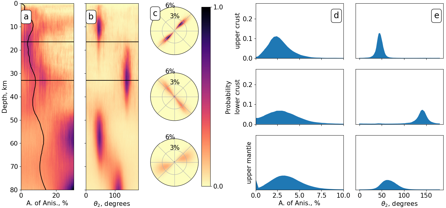
Figure 9 shows an example of inversion of a set of beamforming measurements below the Dinarides (location: ∼45.3°N–16.3°E). The ensemble solution is shown in the left panels, where the probability of a given amplitude range and direction range for shear-wave anisotropy is shown at each depth. However, this way of displaying the posterior distribution does not show correlations and trade-offs between anisotropy amplitude and direction. Such plots do not show whether the sampled profiles contain thin isotropic layers, thin layers with strong anisotropy, or thick layers with small anisotropy.
To extract some key features from this complex probabilistic solution, Soergel et al. [2023] proposed to show the distribution of integrated anisotropy over a given depth range. The integration was defined as in Romanowicz and Yuan [2012], and carried out over three specific depth ranges with a meaningful sense (upper crust, lower crust, uppermost mantle). The distribution for the amplitude and direction of the anisotropy integrated over the three layers is shown in the right panels.
This visualisation makes it possible to see the correlations between fast direction and amplitude of anisotropy in each depth interval. Note that isotropic layers decrease the average level of anisotropy. Additionally, integrating anisotropy over several layers with different fast directions can also lead to anisotropy amplitudes smaller than expected. This explains the differences between the distribution of local anisotropy (left panels), and integrated anisotropy (right panels).
4. New information on the greater Alpine region
One of the main motivations behind the AlpArray initiative was to bring the resolution of seismic tomography closer to the spatial density of geological data over the entire Alpine belt, with the aim of increasing resolution of three-dimensional geological models at lithospheric scale. The methodological developments described in Section 2 have made a valuable contribution to this aim, in particular by providing new insights into the geometry of the crust-mantle boundary. A team of geologists and geophysicists is now working on exploiting the shear-wave velocity models derived by Nouibat et al. [2022a] and Nouibat et al. [2023] to build a 3-D structural model of the Western Alps [Bader et al. 2023]. All available geometrical (digital elevation model), geological (structural and geological maps) and geophysical (3-D Vp and Vs models, DSS profiles, Moho models from seismic and gravity modeling/inversion, etc.) have been integrated and mixed in a geomodeling software, which provides a common framework and checks the geometrical coherence of geological interpretations of geophysical data [Calcagno et al. 2008]. The resolution of Nouibat et al. [2022a]’s model was sufficiently fine to allow Sonnet et al. [2023] to interpret a lateral Vs change in the subducted European lower crust as indication for the transition from amphibolite to granulite based on petrophysical data on Alpine rocks.
A depth map of the iso-velocity surface Vs = 4.2 km/s extracted from the model by Nouibat et al. [2023] is shown in Figure 10. As explained in Section 2.4, a composite depth map of velocity surfaces 3.8, 4.1 and 4.3 km/s would be a better proxy of the three Moho boundaries for the Ivrea body, the Ligurian basin, and Eurasia and Adria outside the Ivrea body region. The Vs = 4.2 km/s surface is therefore only an easy-to-calculate compromise. Since the velocity gradient is generally strong between 4.1 and 4.3 km/s, Figure 10 well illustrates lateral changes in Moho depth beneath the Alps revealed by our ambient noise tomography studies. The purple arrows highlight an ∼8 km step in the European Moho with SSW–NNE orientation beneath the external crystalline massifs of the Western Alps, from Pelvoux to Mont Blanc. This orientation suggests that the Moho step might be a major lithospheric structure inherited from the Variscan orogeny. It had never been imaged before, even by the ECORS-CROP deep reflection profile, which showed reflections from the lower crust only west of the Belledonne external crystalline massif [e.g., Nicolas et al. 1990; see also Supplementary Figure S3 in Paul et al. 2022]. The Vs models of Zhao et al. [2020], Nouibat et al. [2022a], and Nouibat et al. [2023] have confirmed the subduction of the European lithosphere beneath Adria, which is documented in Figure 10 by the dark blue areas (depth > 60 km). The CIFALPS cross-sections in Figures 3d–f document this continental subduction more precisely, with a European Moho reaching 75–80 km depth. Figure 10 also highlights the strong and rapid Moho depth changes along the belt strike, with maximum depths located right beneath the Insubric line (IL in Figure 10, also named Periadriatic fault further east) which marks the western and northern boundary of the undeformed Adria microplate [Handy et al. 2010]. The 3-D detailed geometry and internal structure of the Ivrea body are also important new findings of our ambient noise tomography studies. For example, the “inverted Moho” highlighted by receiver function sections (InvM in Figure 3b, dotted thick grey line in Figure 3e) is explained by the overthrusting of the Ivrea mantle slice of Adriatic origin onto the lower velocity European crust. This boundary was imaged a few tens of km north of the CIFALPS line by wide-angle reflections of the ECORS-CROP complementary experiment [ECORS-CROP Deep Seismic Sounding Group 1989]. It was interpreted as the top of a second mantle slice beneath the Ivrea body, while the polarity of converted signals in receiver function studies and ambient noise tomography studies have proven that this reflector is the base of the Ivrea body (single) mantle slice [Zhao et al. 2015; Paul et al. 2022].
Depth map of the iso-velocity surface Vs = 4.2 km/s, extracted from the wave-equation ambient noise tomography model of Nouibat et al. [2023]. The continuous and dotted black lines are the main geological boundaries and faults, similar to Figure 1. The purple arrows highlight the Moho step located beneath the external crystalline massifs of the Western Alps. The dashed white line outlines the top of the high-velocity, peridotitic core of the Ivrea body, which appears as a dark blue spot in Figures 3d–f. Ad: Adria; CA: Central Alps; EA: Eastern Alps; Eu: Eurasia; IL: Insubric line; Li: Ligurian basin; WA: Western Alps. Modified from Nouibat et al. [2023].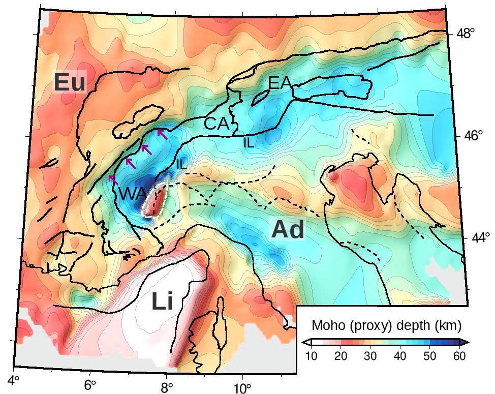
In the Ligurian basin, the wave-equation ANT model with elastic–acoustic coupling by Nouibat et al. [2023] has provided new images of the basin margins and new estimates of sediment thickness with potential inferences on tectonic models of basin formation. On Ligurian Moho depth, the recently published ANT Vs model by Magrini et al. [2022] exhibits significant differences from the Vs model by Nouibat et al. [2022b], with 15–18 km crustal thickness along the basin axis in Magrini et al. [2022]’s model and 12 km in Nouibat et al. [2023]’s. As explained in Section 2.4, the thinner crust of Nouibat et al. [2022b] is fully consistent with the P-wave velocity model derived from the refraction-reflection profile LOBSTER-P02 of Dannowski et al. [2020] along the Ligurian basin axis. The difference in Moho depth estimates between Nouibat et al. [2022b, 2023] and Magrini et al. [2022] may be due to different ray coverages in the Ligurian basin, as Magrini et al. [2022] did not use AlpArray OBS data.
Very little information was available on the anisotropy of the crust and upper mantle beneath the Alpine region prior to the works described in Section 3. Kästle et al. [2022] and Soergel et al. [2023] have mapped azimuthal anisotropy of Rayleigh wave phase velocity using ambient noise records of the AASN and permanent seismic stations, and two different methods, Eikonal and beamforming. Their azimuthal anisotropy maps are broadly similar at all periods, except at the periphery of the study area, probably due to differences in ray coverage (see examples at 15 and 40 s period in Figures 5 and 7). The Bayesian inversions for azimuthal anisotropy distribution with depth by Soergel et al. [2023] have shown that the anisotropic structure cannot be easily inferred from maps at individual periods. Spatially coherent anisotropy patterns are only visible in the upper half of the crust, with fast-velocity directions mostly parallel to the strike of the belt and amplitudes of 1–2% [see Figure 14 in Soergel et al. 2023]. By contrast, fast-velocity directions are mostly perpendicular to the belt in the lower half of the crust and uppermost mantle, with strongly varying amplitudes and no large-scale spatial pattern. This contrast between the shallow and deep layers suggests that Alpine deformation has only impacted the upper crust, through oriented crack and fractures, while the lower crust and upper mantle bear the imprint of more ancient processes. A single region located northwest of the Jura mountains displays coherent NE–SW fast velocity directions from the upper crust to the upper mantle, and rather strong amplitudes (∼1%) in the lower crust. This orientation suggests that the observed anisotropy in that area outside the Alps may be of Variscan origin, and unaffected by the Alpine orogeny. Soergel et al. [2023] highlight the general disagreement between the fast-velocity directions they measured in the upper mantle and the fast directions measured from the splitting of core-refacted XKS teleseismic phases [e.g., Hein et al. 2021]. This may indicate that the source of XKS splitting is located deeper than the lithospheric mantle, either in the asthenosphere or in the subduction slabs.
When applied to Rayleigh and Love dispersion curves measured in the Alpine region, the flexible parameterization of Bayesian inversion allowed Alder et al. [2021] to produce maps of radial anisotropy differing from previous large-scale studies that suggested the presence of significant radial anisotropy everywhere in the European crust and shallow upper mantle [e.g., Zhu et al. 2015]. Instead, they observed that radial anisotropy is mostly localised beneath the Apennines while most of the crust and shallow upper mantle is isotropic in other parts of Europe. Thanks to synthetic tests, they attributed this difference to trade-offs between radial anisotropy and thin (hectometric) layering in previous studies based on least-squares inversions and long period data (>30 s). In contrast, Alder et al. [2021]’s approach involved a massive dataset of short period measurements and a Bayesian inversion that accounts for thin layering. They showed that the positive radial anisotropy (VSH > VSV) observed in the lower crust of the Apennines could not result from thin layering, but rather from ductile horizontal flow in response to the strong flexure of the Adriatic plate induced by doubly-vergent subduction.
5. Conclusions
The Alpine broadband seismic networks, including permanent stations and the temporary AlpArray seismic network have provided an optimal dataset for the development, improvement, and application of ambient-noise-based imaging methods. High station density and homogeneous coverage were key elements for these methodological improvements.
The overarching goals of our work were to improve observations when needed, move towards a probabilistic framework for inversion and interpretation, and adapting full waveform modelling in the forward problem. On the observational side, the work focused on (a) developing suitable techniques to combine OBS and land observations through higher order correlations, (b) improving our understanding of systematic errors made when measuring surface wave azimuthal anisotropy, and (c) applying and adapting beamforming techniques to seismic noise correlations to estimate surface wave anisotropy.
For the inversions, a Bayesian framework was applied both to 2-D inversions for group velocity maps [Nouibat et al. 2022a], and to 1-D depth inversions for elastic structure [Lu et al. 2018; Zhao et al. 2020; Alder et al. 2021; Soergel et al. 2023]. Particular efforts [Alder et al. 2021; Soergel et al. 2023] were made on the extraction of robust anisotropic parameters which are meaningful in a geologic/tectonic sense. Wave-equation ambient noise tomography studies by Lu et al. [2020] and Nouibat et al. [2023] have further improved ANT models by accounting for the physics of seismic wave propagation. The introduction of elastic–acoustic coupling at the seabed has enabled Nouibat et al. [2023] to improve the imaging of shallow layers below the sea. All of these developments led to improved models of the crust and uppermost mantle on the scale of the greater Alpine area (see Section 4).
The link between the overarching goals is naturally increasing because of the strong link between observational errors and the estimation of model resolution within a probabilistic inversion framework. In such a framework, the inversion provides not a single Earth model, but an ensemble of models obtained whilst taking into account uncertainties of inverted data. In this context, reliable error estimates of observables become objectively tied to the estimation of model uncertainties [Gallagher et al. 2009; Sambridge et al. 2013]. Also, the ensemble of models can be explored based on scientific questions (for example “What is the probability that the lower crust beneath the Apennines has significant radial anisotropy of crystallographic origin?”) [Curtis 1999; Meier et al. 2007; Zhang and Curtis 2021].
Note also that the Bayesian framework allows to include independent information from geology, mineralogy, or other geophysical methods such as gravimetry. This can be done through the definition of the a priori distribution, or through the joint inversion of different datasets. Including other data types sensitive to P-wave structure (body waves) would be very useful for geological interpretation, as P and S waves have different sensitivities to different rock types, for example to hydrated minerals. In this context, full waveform inversion has the benefit to model the entire wavefield without having to preliminary extract and separate different data types (arrival times, phase velocities, splitting parameters, etc.), and three-dimensional variations of the entire elastic tensor can be directly reconstructed, including Vp, Vs and anisotropy. However, full waveform tomography in a fully non-linear Bayesian framework is still a prospect for the future, due to the computational cost of the forward model.
Within the framework of the AlpArray experiment, other noise-based methods were developed. For crustal imaging, it is becoming feasible to image coda-Q [Soergel et al. 2020], overcoming the difficulty of obtaining reliable amplitudes of noise correlations. This method makes it possible to estimate coda-Q at longer periods than those accessible through local earthquake estimates, but the method needs to be further developed to fully understand the meaning and reliability of the observed coda-Q values. The dense data coverage of the Alps also served the purpose of improving methods to extract body waves (reflections from mantle discontinuities) from seismic noise correlations [Pedersen et al. 2023; Lu et al. 2023].
The methods developed within the framework of the AlpArray experiment can naturally be applied and further improved within the framework of other dense and large-scale seismic arrays, such as the recently started AdriaArray experiment which significantly extends the area of high station density around the Adriatic plate, from the French Massif Central in the west to the Carpathians in the east [Kolínský et al. 2023; https://orfeus.readthedocs.io/en/latest/adria_array_main.html].
Declaration of interests
The authors do not work for, advise, own shares in, or receive funds from any organization that could benefit from this article, and have declared no affiliations other than their research organizations.
Funding
A large part of the studies described here were conducted within the AlpArray-FR project funded by Agence Nationale de la Recherche, France (contract ANR-15-CE31-0015), and Labex OSUG@2020 (Investissement d’Avenir, ANR-10-LABX-56). TB, CA and DS were funded by the European Research Council under the European Union Horizon 2020 research and innovation program (grant agreement 716542 – TRANSCALE). AP’s work on the Alps is currently funded by project LisAlps (contract ANR-20-CE49-0007). EK is funded by the German Science Foundation DFG (SPP-2017, Project Ha 2403/21-1).
Acknowledgments
We are grateful to our colleagues, Laurent Stehly, Romain Brossier, and Eric Debayle who co-supervised YL’s, CA’s and AN’s Ph-D theses with AP and TB, and have made major contributions to much of the work presented here. Liang Zhao (IGG-CAS Beijing) is also acknowledged for his decisive contributions to this work. This paper was partly conceived during the Cargèse 2022 school on “Passive imaging and monitoring in wave physics: from seismology to ultrasound”, in which AP took part. We would therefore like to thank the organizers, in particular Michel Campillo and Nikolaï Shapiro for encouraging us to write it. We acknowledge detailed and constructive comments by two anonymous reviewers that helped improving the manuscript, and editorial handling by Andrew Curtis. Without high-quality, open data, such work is impossible. We therefore gratefully thank the operators of the European permanent seismic networks who make their data available through EIDA (http://www.orfeus-eu.org/eida), the AlpArray Seismic Network Team who operated the AASN (Z3-2015 network) and the CIFALPS Team who operated the CIFALPS experiments (YP-2012 and XT-2018 networks).