Modelling diffusion in a heterogeneous rock matrix with a time-domain Lagrangian method and an inversion procedure

Frédérick Delay; Gilles Porel; Paul Sardini

doi:10.1016/S1631-0713(02)01835-7

Résumés

Anglais
Français

A Lagrangian method in time domain is proposed to solve transport by diffusion over large grids such as those extracted from autoradiographs of rock samples. The method is rapid and well suited to simulate out-diffusion experiments in a heterogeneous rock matrix. By coupling with a Gauss–Newton optimiser, it is possible to identify automatically the diffusion coefficients of porous areas in the matrix. This offers a more comprehensive view of a potential transport of contaminants, e.g., after a leak from an underground repository site.

Nous présentons une nouvelle méthode lagrangienne dans le domaine des temps pour le calcul de la diffusion sur des maillages de grande taille, comme ceux extraits des autoradiographies d'échantillons de roche. La méthode est bien adaptée aux simulations d'expériences de rétro-diffusion sur des roches hétérogènes. L'association à une optimisation de type Gauss–Newton permet d'identifier les coefficients de diffusion de la matrice rocheuse. Ceci nous procure une vue plus éclairée sur le transport de polluants, par exemple en cas de fuites sur un site de stockage souterrain.

Version abrégée

Les laboratoires souterrains développés pour l'étude de faisabilité de sites de stockage sont confrontés à des calculs de sûreté, qui nécessitent la connaissance des vitesses de diffusion dans la matrice rocheuse. Pour cela, les expériences de rétro-diffusion en laboratoire sont un outil précieux. Après avoir saturé l'échantillon par un fluide enrichi en traceur (soluté inerte ou radioélément) on le plonge dans le même fluide, mais initialement exempt de traceur. La rétro-diffusion s'effectue de la matrice rocheuse vers la solution, dont on suit l'évolution de la concentration au cours du temps. Si le soluté est remplacé par un radioélément, il est alors possible, en marge des expériences de diffusion, de procéder à des autoradiographies. Ces dernières fournissent des images 2D de la porosité connectée de l'échantillon. On peut ainsi mettre en évidence l'hétérogénéité de la porosité en raison, par exemple, d'une altération différentielle des minéraux, ou encore l'existence de micro-fissures et de joints de grains ouverts (Fig. 1). Des outils d'analyse d'image appliqués aux autoradiographies permettent l'extraction de grilles qui, pixel par pixel, reflètent la géométrie de l'espace poreux dans la roche. L'opportunité est ainsi offerte de simuler numériquement un transport par diffusion sur ces grilles, avec, pour premier intérêt, la prise en compte immédiate de l'hétérogénéité. C'est un point crucial, qui fait défaut aux méthodes couramment utilisées, basées sur des solutions analytiques pour l'interprétation des expériences de rétro-diffusion.

Figure 1
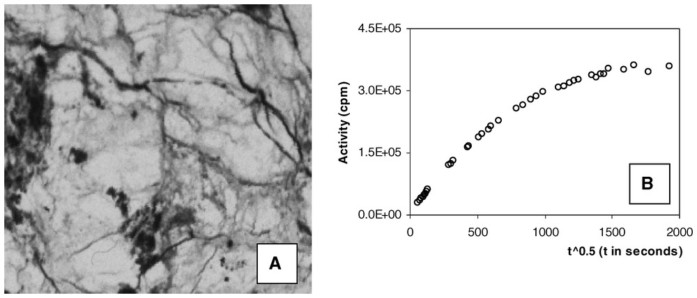
A. Example of autoradiography from a sample of the Kivetty granite (Finland). B. Example of out-diffusion curve (concentration = activity in counts per minute).
A. Exemple d'autoradiographie d'un échantillon du granite de Kivetty (Finlande). B. Exemple de courbe de rétro-diffusion (concentration = activité en coups par minute).

Nous avons développé une nouvelle méthode de calcul particulièrement bien adaptée au cadre précédent. Il s'agit d'un calcul lagrangien dans le domaine des temps. On peut démontrer (expressions (1) à (5)) qu'en retravaillant l'équation de diffusion dans son formalisme « volumes finis », il est aisé de calculer : (1) la probabilité de transition d'une particule entre un pixel et ses voisins immédiats ; (2) la durée aléatoire du saut diffusif entre deux pixels voisins. À l'usage, la méthode s'avère nettement plus rapide qu'un marcheur aléatoire classique dont on suit le déplacement dans l'espace au cours du temps. En effet, la méthode en temps assure à chaque pas de calcul que la particule passera d'un pixel à un voisin. Avec un marcheur aléatoire classique, le nombre de sauts par pixel doit être beaucoup plus important, afin de mimer correctement le phénomène de diffusion. La méthode TDD (Time Domain Diffusion) a été couplée à une optimisation de type Gauss–Newton (expressions (7) à (12)), afin de résoudre un problème inverse, soit, dans le cas présent, l'identification des coefficients de diffusion apparents distribués dans la matrice rocheuse (la diffusion apparente correspond à la diffusion de pore multipliée par un coefficient de retard, si le soluté s'adsorbe selon un équilibre instantané sur le solide). La méthode cherche le meilleur jeu de coefficients, afin de minimiser les erreurs entre courbes de rétro-diffusion simulées et observées. L'algorithme nécessite l'estimation du jacobien des erreurs sus-citées, le calcul convergeant d'autant plus vite vers la solution que cette estimation est précise. Le cadre lagrangien de la méthode TDD impose de procéder par perturbation, ce qui est a priori moins efficace qu'une dérivation analytique. Cela étant, l'exemple synthétique proposé (Fig. 2) est résolu avec succès en 12 itérations. Des améliorations restent possibles. Ainsi, certaines courbes de rétro-diffusion montrent des segments distincts, dont l'essentiel est issu de zones de porosité bien individualisées dans la matrice. En marquant les particules issues de ces zones, il serait possible de mieux focaliser la procédure inverse et notamment d'améliorer sa sensibilité en ne lui faisant chercher que le (ou les) paramètres qui influence(nt) vraiment le calcul à un endroit particulier de la courbe de rétro-diffusion. Notons que les travaux en cours devraient bientôt permettre de dériver analytiquement les expressions du jacobien par un calcul en temps et accélérer la convergence. Utiliser des procédures d'inversion est un bon moyen de limiter la subjectivité inhérente aux ajustements « à la main ». En réinterprétant les nombreuses expériences disponibles, on peut espérer progresser, fiabiliser et rendre prédictives les études menées notamment pour la sûreté des sites de stockage.

Figure 2
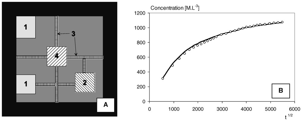
A. Calculation grid of a synthetic problem of out-diffusion. Grey areas are impervious (porosity = 0), areas numbered from 1 to 4 have porosity values of 0.25, 0.1, 0.3, 0.15, respectively, and the black rim corresponds to the external fluid. B. Reference out-diffusion curve (solid line) and the best solution found by Gauss–Newton inversion (dots).
A. Grille d'un problème fictif de rétro-diffusion. Les zones en gris sont imperméables (porosité = 0), les zones numérotées de 1 à 4 ont des valeurs respectives de porosité de 0,25, 0,1, 0,3, 0,15, la couronne noire correspond à la solution externe. B. Courbe de rétro-diffusion de référence (ligne) et solution optimale de l'inversion de Gauss–Newton (points).

1 Introduction

The need for underground repositories has given rise to a number of studies of flow and transport in low-permeability rocks. To isolate the contaminants from the environment, crystalline rocks or clay are considered the most suitable. These media often have large-scale fractures and the safety calculations for the so-called ‘far field’ have to take into account the up-scaling of the flow properties [10] and transport in the fracture networks [1,9]. At the scale of the ‘near field’, it is assumed that the main mechanism affecting potential leaks is diffusion through the rock matrix, which is always heterogeneous. In crystalline rocks, the matrix consists of different grains more or less weathered according to their mineralogy. Micro-cracks and open inter-grain joints may also exist. This results in heterogeneous pore-space patterns and therefore variable pore diffusion coefficients. In clays, the damaged zone around the wells and galleries is large enough to contain unevenly distributed areas of open and connected porosity. Diffusion velocities can be measured either in the field [8,11] or in the laboratory, on core samples [2,12]. Measurements on cores are more accurate, because it is easier to control the experimental conditions, and a classical method is to perform out-diffusion experiments, whose principle may be described as follows. The core is plunged into a fluid doped with a solute and is left in the solution during a sufficiently long period to evenly saturate the rock. Afterwards, the sample is out-leached by plunging it into a vessel containing the same liquid, but without the solute. Out-diffusion of the solute occurs and the concentration of the external solution is monitored. An interesting variation is to replace the solute by a radioactive element, for instance, a MethylMethAcrylate resin doped in ¹⁴C. With this method, one can obtain autoradiographs of the sample, which basically provide 2D images of the connected porosity. The grey level of each pixel of the image can be converted into a porosity value by comparison with calibrated sources radiographed with the sample (for details, see [3]). An example of autoradiograph and out-diffusion curve from the Kivetty granite (Finland) is shown in Fig. 1. Usually, the out-diffusion curves are interpreted by analytical solutions that are exact in the context of a homogeneous diffusion. In the early times of the experiment, the homogeneous assumption should yield an increasing linear behaviour of the concentration curve with respect to the square root of time [4]. As shown in Fig. 1, this interpretation is not acceptable because the heterogeneous porosity of the rock generates a very complex convex curve.

By using image processing on the autoradiographs, we are able to build calculation grids where each pixel is associated with a known porosity value and an unknown apparent diffusion coefficient. Note that the apparent diffusion is the pore diffusion multiplied by a retardation factor when sorption onto the solid occurs with instantaneous equilibrium. In the following, it is assumed that there is no sorption and, for the sake of simplicity, the pore diffusion will be referred to as diffusion. Numerical simulations of the diffusion can be made, as well as attempts at identifying the values of the diffusion coefficients. By using 2D or reconstructed 3D geometry, one can fit the complex experimental curves and enhance the predictive capabilities of the model, because heterogeneity is accounted for, both in terms of the pore space geometry and the diffusion properties. This work demands cumbersome calculations, because a precise geometry of the pore space requires grids with sometimes several million pixels. The aim of the present work is to propose a new numerical method, much more rapid than classical ones to solve the heterogeneous diffusion. It is also coupled with a mathematical optimisation procedure to find the diffusion coefficients. Finally, a synthetic example is given for illustration purpose.

2 The direct problem: solving diffusion in a heterogeneous rock matrix

As mentioned above, the computation grids may count millions of unknowns and to avoid handling the huge and sparse matrices of the Eulerian methods, we have chosen the Lagrangian approach. In this context, the classical Random Walk (RW) method moves particles by jumps in space and over pixels that correspond to the connected porosity [5]. Since the initial concentration of the out-diffusion experiment is constant over the whole porosity, a given number of particles per porous pixel is required to obtain a relevant representation (at least one particle for the less porous pixel of the medium). Moreover, RW needs a minimum of 2–4 jumps for each particle and in each pixel for an accurate representation of the diffusive transport. These constraints argue against the classical RW, leading us to develop a more rapid method using particles in the time domain.

The principle is to calculate the diffusion time needed by a particle to jump from centre to centre of neighbouring pixels. The method is partly inspired by and modified from previous attempts in petroleum engineering to solve the steady-state flow equation [7]. The diffusion equation in heterogeneous media is:

\frac{\partial (ϕ C)}{\partial t} = \nabla \cdot (ϕ \underline{\underline{D}} \cdot \nabla C)

(1)

where φ is the porosity [−],

\underline{\underline{D}}

the diffusion tensor [L²T⁻¹] and C the concentration of solute [ML⁻³]. Assuming a diagonal and isotropic diffusion tensor and using a finite-volume formalism, this equation may be rewritten as:

ϕ_{i} V_{i} \frac{\partial C_{i}}{\partial t} = \sum_{j} S_{ij} {(ϕ D)}_{ij} \frac{C_{j} - C_{i}}{L_{ij}}

(2)

with i the index referring to pixel i and j referring to the pixels that are the direct neighbours of i. C_α is the mean concentration in pixel α (α=i,j); L_ij the lag distance between the centres of pixels i and j, S_ij the total area of the interface between pixels i and j, V_i the total volume of pixel i and

{(ϕ D)}_{ij}

the harmonic mean of the product porosity × diffusion coefficient between pixels i and j. Knowing that a partial derivative with respect to time is a material derivative in the Lagrangian context and denoting

S_{ij} {(ϕ D)}_{ij} / L_{ij}

as b_ij, (2) can be rewritten in the form:

ϕ_{i} V_{i} \frac{d C_{i}}{d t} = - [\sum_{j} b_{ij}] C_{i} + \sum_{j} b_{ij} C_{j}

(3)

which is equivalent to:

\frac{ϕ_{i} V_{i}}{\sum_{j} b_{ij}} d (\log (C_{i})) = - d t + \frac{\sum_{j} b_{ij} C_{j} / C_{i} d t}{\sum_{j} b_{ij}}

(4)

The dimensional analysis of the second term of the right-hand side shows that expression (4) may be rewritten as separate equations, in the form: $d t = - (ϕ_{i} V_{i} / \sum_{j} b_{ij}) d (\log (C_{i}))$ with an occurrence probability p_ij such as: p_ij=b_ij/∑_jb_ij. Note that b_ij is of dimension [L³T⁻¹], and therefore the probability p_ij corresponds to the fraction of the volumetric flux that passes by diffusion from i to j. In other words, a particle present at the centre of pixel i will jump to the centre of pixel j with a transition probability p_ij and the diffusion time from i to j is given by:

t_{i \to j} = - \frac{ϕ_{i} V_{i}}{\sum_{j} b_{ij}} \log (u_{01})

(5)

with u₀₁ a random number from a uniform distribution between 0 and 1. The transition time t_i→j follows an exponential distribution and if the pixel j is impervious, the transition probability p_ij cancels out, which avoids a jump from i to j. This Time Domain Diffusion method (TDD) makes the particle move systematically from one pixel to one of its neighbours. The calculation is therefore much more rapid than a classical RW, especially for problems with diffusion coefficients spanning several orders of magnitude. As stated earlier, RW necessitates a minimum of 2–4 jumps per pixel and when applied to the most diffusive pixels of the grid, this implies hundreds of jumps for the less diffusive pixels.

The TDD method is based on a finite-volume formalism and is therefore not free from truncation errors, even if the calculation is performed in time. These errors are of the fourth order with respect to space coordinates or equivalently, of the second order with respect to time. Typically, this error for a jump of size Δx is:

ϵ_{Δ} = - \frac{D Δ x^{2}}{12} \frac{\partial^{4} C}{\partial x^{4}} = - \frac{Δ x^{2}}{12 D} \frac{\partial^{2} C}{\partial t^{2}}

(6)

and in concrete applications, i.e. with average values of

D = 10^{- 11} m^{2} s^{- 1}

and Δx=10⁻⁴ m, we have found it negligible.

3 Inversion of the direct problem: identification of the diffusion coefficients

It can be assumed that the image processing of autoradiographs provides the porosity value of each pixel, but the diffusion coefficient remains unknown. Note, however, that the porosity could also be identified, for instance, if the confidence in the image is poor. The inversion might refine the knowledge of the porosity values with the processed image acting as a preconditioning in setting the range of possible values for each grey level. In the following, the problem is simplified by focusing the inversion on the diffusion coefficients. It is obvious that we cannot identify one specific value for each pixel: this would lead to an ill-posed problem with thousands of parameters as compared to limited observations, i.e. the experimental out-diffusion curve. A parameterisation able to strongly reduce the set of the sought parameters is required. In crystalline rocks, the variations of porosity are mostly the consequence of differential weathering and micro-deformations, such as kinks and cracks, which affect the grains, specifically according to their mineralogy. Thus, a strong link exists between the porosity value, the internal pore geometry (constrictivity and tortuosity of pores), and the medium in which it develops. Knowing this, a simple and efficient parameterisation consists in assigning a constant and unknown diffusion coefficient to each grey level of the image. There are as many parameters to identify as grey levels, i.e. a maximum of eight in current applications (the number of thresholds in processing the autoradiographs could be increased, ongoing work shows that 8 to 12 grey levels are sufficient on most images).

The inversion is performed following an indirect approach, i.e. by seeking the parameters iteratively until a criterion of closeness between the observed and the simulated out-diffusion curves is reached. If ${\underline{d}}^{k} = {d_{1}^{k}, \dots, d_{p}^{k}}$ denotes the vector of the p parameter values at iteration k and ${\underline{ξ}}^{k} = {ξ_{1}^{k}, \dots, ξ_{n}^{k}}$ the vector of the n sampled errors between observed and simulated concentrations, the closeness criterion minimises a classical least-square function:

F ({\underline{d}}^{k}) = {\underline{ξ}}^{k T} \cdot {\underline{ξ}}^{k}

(7)

with ^T the transposition operator. The Taylor development of F with respect to

\underline{d}

may be written as:

F ({\underline{d}}^{k + 1}) = F ({\underline{d}}^{k}) + {({\underline{d}}^{k + 1} - {\underline{d}}^{k})}^{T} \cdot \nabla F ({\underline{d}}^{k}) + \frac{1}{2} {({\underline{d}}^{k + 1} - {\underline{d}}^{k})}^{T} \cdot \nabla^{2} F ({\underline{d}}^{k}) \cdot ({\underline{d}}^{k + 1} - {\underline{d}}^{k})

(8)

with ∇F and ∇²F, the gradient vector (∂F/∂d_j) and the Hessian matrix

(\partial^{2} F / \partial d_{i} \partial d_{j})

, respectively. The optimisation techniques using a ‘descent’ direction assume that

F ({\underline{d}}^{k + 1})

is stationary, i.e.

\nabla F ({\underline{d}}^{k + 1}) = 0

. Cancelling the gradient derived from the second-order development in (8) gives the general recursive form to calculate

{\underline{d}}^{k + 1}

as a function of

{\underline{d}}^{k}

\nabla^{2} F ({\underline{d}}^{k}) \cdot ({\underline{d}}^{k + 1} - {\underline{d}}^{k}) = - \nabla F ({\underline{d}}^{k})

(9)

The Gauss–Newton method uses the exact expression for the gradient and an approximation for the Hessian:

\nabla F ({\underline{d}}^{k}) = J_{ξ^{k}}^{T} \cdot {\underline{ξ}}^{k}; \nabla^{2} F ({\underline{d}}^{k}) = J_{ξ^{k}}^{T} \cdot J_{ξ^{k}}

(10)

with J_ξ the n×p Jacobian matrix of

\underline{ξ}

: (∂ξ_i/∂d_j).

This method has proven its capacity to solve inverse problems with few parameters [6]. The reason may be that the method corresponds to the least-square resolution of the general linear approximation: $f (b) = f (a) + (b - a) (\partial f / \partial x)$ . Applied to the error vector $\underline{ξ}$ as a function of the parameter vector $\underline{d}$ , this gives:

{\underline{ξ}}^{k + 1} - {\underline{ξ}}^{k} = J_{ξ^{k}} \cdot ({\underline{d}}^{k + 1} - {\underline{d}}^{k})

(11)

Cancelling

{\underline{ξ}}^{k + 1}

and using a least square resolution of the n×p system in expression (11) yields:

- J_{ξ^{k}}^{T} \cdot {\underline{ξ}}^{k} = (J_{ξ^{k}}^{T} \cdot J_{ξ^{k}}) \cdot ({\underline{d}}^{k + 1} - {\underline{d}}^{k})

(12)

which is equivalent to expressions (9) and (10).

When the optimisation is completed, the Gauss–Newton method offers directly, as a by-product, the sensitivity of the model to the parameters. Each term (∂ξ_i/∂d_j) of the Jacobian matrix can be viewed as the local sensitivity (in ξ_i) to the parameter d_j. The terms of J_ξ^T·J_ξ are: $\sum_{λ = 1}^{n} {(\partial ξ_{λ})}^{2} / \partial d_{i} \partial d_{j}$ and can thus be interpreted as measures of the global sensitivity of the model. The diagonal terms of the matrix are proportional to the variance of the sensitivity to d_i, the out-diagonal terms are proportional to the covariance of the sensitivity to d_i and d_j. It is obvious that the less sensitive the model is to a parameter, the larger the uncertainty on the parameter value. The calculation of the Jacobian matrix is described in the following section.

4 An example of inversion

The example proposed below is a synthetic one, built for illustration purposes and to demonstrate the relevance of the whole inversion procedure, i.e. the TDD transport simulator and the Gauss–Newton method for identifying the parameters. The computation grid is shown in Fig. 2a. It encloses four types of zones with different porosities and diffusion values in a rock matrix, plus the external fluid. Three of these zones are porous patches that could mimic areas of different mineralogy and, as stated before, they are affected by differential weathering (porosity of 0.1, 0.15, 0.25, see Fig. 2). These patches are connected to each other and to the edges of the sample either directly, or by thin stripes that may represent partly filled cracks in the matrix (porosity of 0.3). The total grid size is 100×100 square pixels of 5×10⁻⁴ unit length on a side. In view of the grid, it can be foreseen that the out-diffusion curve is likely to show variations in the slopes of the concentration versus time. This is the logical consequence of the variable connectivity between the pore space and the edges of the sample. Some highly diffusive patches are in direct contact with the external fluid and will contribute most to the concentration curve in early times. On the other hand, the patches with low diffusion or those merely connected to the edges by thin stripes contribute to a delayed concentration increase. The direct problem was solved to get a reference curve for the inversion with the following set of diffusion coefficients: {2×10⁻¹¹,5×10⁻¹³,2×10⁻¹¹,2×10⁻¹²} [L²T⁻¹] ranked according to the indexes of zones in Fig. 2. The initial condition of a constant concentration at any location in the matrix was set up by placing 10 particles in each of the less porous pixels, the other pixels being filled according to this value (e.g., 10 particles for a porosity of 0.1→15 particles for 0.15). With these settings, the direct simulation is performed in less than 10 seconds with a Pentium 2 GHz. The reference out-diffusion curve is shown in Fig. 2b.

To obtain an operational Gauss–Newton inversion, the Jacobian matrix (see Section 3) must be calculated. Contrary to Eulerian models, the Lagrangian framework of the transport simulator (see Section 2) jeopardizes the chance to derive analytically the Jacobian matrix in (12). It was thus processed numerically and the term-by-term evaluation of the Jacobian can be represented by:

\frac{\partial {\underline{ξ}}^{k}}{\partial d_{j}^{k}} \approx \frac{\underline{ξ} (d_{j}^{k} + δ d_{j}) - \underline{ξ} (d_{j}^{k})}{δ d_{j}}

(13)

with δd_j a small perturbation in the value of the parameter d_j.

In theory, the perturbation should tend toward zero for the best estimation, but the stochastic nature of Lagrangian computations prohibits the use of very small perturbations. With a reasonable number of particles, two direct calculations with the same parameters may show slightly different results. A relative difference of 1% or so on the concentrations is negligible when the problem is to simulate a transport scenario, but for an inversion, it imposes to set the δd_j values so that they induce visible modifications of the concentrations as compared to the uncertainty from the direct calculation. The perturbations were therefore set to 10% of the current parameter values at each iteration. Note that for each perturbed calculation, we did not keep the same chain of generated random numbers u₀₁ (in expression (5)) used to move the particles. The first reason is that a perturbation on a parameter modifies both the transition probability and the transition time distribution from pixel to pixel. Thus, keeping the same random number for a transition has no physical consistency. In addition, this procedure has shown to be cumbersome in terms of storage capacity and there is no significant gain in computation costs.

The starting point of the inversion was set at 5×10⁻¹² [L²T⁻¹] for any porous zone and the diffusion coefficient for the external fluid was assumed to be known (10⁻¹⁰ L²T⁻¹). The Gauss–Newton algorithm finds its optimal solution in 12 iterations and yields the following diffusion coefficients {1.85×10⁻¹¹,1.62×10⁻¹²,1.52×10⁻¹¹,3.45×10⁻¹²}. Whereas areas 1, 3, and 4 are found with precision, area 2 is poorly identified. The reason is that the particles from area 2 contribute weakly to the out-diffusion curve, since (1) the area is not well connected to the edges of the sample and initially encloses few particles, (2) the low diffusion coefficient causes these particles to be present in the flat part of the concentration curve (latest times) where the model is not sensitive. This is confirmed by the diagonal of the Jacobian matrix, whose values have been normalized by the optimal parameters to produce something with the dimension of a quadratic error: (∑_λ=1ⁿ(δξ_λ/δd_i)²)d_i². These values are {6.16,2.88,13.4,45.2}×10⁴ [ML⁻³]² and show the model to be less sensitive to parameter #2. Making the starting point vary does not really change anything, except when it is very close to the true solution. This feature is inherent in the inverse problem and not the consequence of the Gauss–Newton optimiser. However, some out-diffusion curves may show different portions, each of them stemming from particles of fairly well identified areas. By adding a flag to these particles, one could focus the inversion on the parameter that is assumed to mainly influence a specific part of the curve. This would increase the speed of convergence and probably, the sensitivity to parameters. We also carried out inversions in a more classical way using an Eulerian finite volume formalism, a Gauss–Newton optimiser and an analytical derivation of the Jacobian matrix (which is straightforward in the Eulerian context). The performance in terms of parameter identification is similar to TDD inversion. However, each direct simulation requires ten times as much computation time as TDD. Even though the analytic Jacobian lowers convergence iterations from 12 to 8, the TDD inversion remains much more rapid than a classical discrete method.

5 Conclusion

Out-diffusion experiments are widely used to assess the safety of potential underground repository sites. We have shown that a comprehensive interpretation of the diffusion through a heterogeneous rock matrix needs intensive computations. We built a Lagrangian simulator in the time domain that is rapid and well suited to transport simulations over grids extracted from autoradiographs of rock samples. The calculations are well conditioned to both the spatial distribution and the local values of the porosity. In addition, the coupling with a Gauss–Newton optimiser makes it possible to seek automatically the diffusion coefficients and lowers the subjectivity of a classical fitting by ‘trial and error’. Further works will focus on how to increase the sensitivity of the inversion to the parameters. For instance, some theoretical developments are in progress to derive the analytical form of the Jacobian matrix and calculate its coefficients by a method similar to TDD. Basically, this improvement does not modify the principle of the Gauss–Newton inversion, but a better estimation of the descent direction would probably lower the number of convergence iterations. Other lines of research also deserve some interest, for instance, adding mechanisms such as sorption with first-order kinetics and handled in the time domain.

Acknowledgements

We are grateful to the ‘French National Program for Research in Hydrology’ for the financial support of this work.