

Version française abrégée
1 Introduction
Le phénomène ENSO (El Niño/Southern Oscillation), habituellement synthétisé au sein de l'indice SOI (Southern Oscillation Index), est l'un des facteurs à l'origine des variations interannuelles de la circulation atmosphérique mondiale [20,25]. Il engendre des effets parfois dévastateurs jusqu'aux hautes latitudes, en modifiant les distributions des pluies et des températures [6,22]. L'Amérique du Sud, en particulier, est depuis longtemps touchée par le phénomène [2]. ENSO affecte l'Amérique du Sud et le Bassin atlantique selon deux types de téléconnexions atmosphériques :
- (i) un événement El Niño crée un décalage vers l'ouest de la zone de convection habituellement centrée sur l'Amazonie, doublé d'une convergence des vents d'est et d'ouest du continent [28] ; les alizés atlantiques sont renforcés par cette zone de convergence et activent ainsi la modeste cellule atmosphérique du bassin atlantique ;
- (ii) cette configuration est accentuée par un blocage des fronts polaires et de son puissant jetstream subtropical dans la région allant du Sud du Pérou au Sud du Brésil [14].
Les conséquences de cette situation sont une pluviométrie anormalement élevée dans la zone de blocage précédente et une sécheresse des zones situées plus au nord, le Nord–Est brésilien et le plateau des Guyanes [12]. Dans l'année qui suit un événement El Niño important, l'Atlantique nord (NA) est généralement caractérisé par une température des eaux de surface (SSTA) anormalement élevée, tandis que l'Atlantique sud (SA) est parfois (et non systématiquement) dans une situation opposée [7]. Au cours des événements La Niña, la partie descendante de la cellule atmosphérique équatoriale atlantique tend à s'affaiblir et à s'étaler. Cela réduit d'autant les alizés de l'Atlantique, déplace vers le sud la zone de convergence intertropicale et accroı̂t la pluviométrie des marges continentales voisines (plateau des Guyanes). Comme illustration de ces mécanismes, nous avons trouvé une corrélation croisée (Cross Correlation Function, CCF) importante entre le SOI et les débits des fleuves de Guyane française. Pourtant, pour ce calcul comme pour les études précitées, nous avons fait une hypothèse (forte ?) selon laquelle un événement isolé d'ENSO est à l'origine d'une réduction de la pluviométrie en Guyane à un autre moment isolé. Nous proposons une nouvelle approche statistique pour examiner les conséquences d'une telle hypothèse, en gardant à l'esprit que nous manipulerons des corrélations et non des causalités.
2 Contexte scientifique
L'hydrologie du plateau des Guyanes a été peu étudiée jusqu'ici [11]. Nos données proviennent de la Guyane française, un département français d'une superficie approximative de 84 000 km2, situé au nord du Brésil sur la côte Atlantique. Nous avons utilisé les débits mensuels de ses deux principaux fleuves (le Maroni et l'Oyapock), enregistrés entre 1954 et 1996 par l'Institut de recherche pour le développement (IRD, ex-Orstom), avec une incertitude moyenne de mesure de 5 %. Par la suite, chacune des deux séries temporelles a été standardisée (de moyenne nulle et d'écart type égal à 1) ; elles ont été moyennées entre elles et désaisonnalisées (divisées par la courbe moyenne sur les 42 années), puis comparées aux indices climatiques précités (SOI, NA et SA). La comparaison SOI/débits montre clairement une corrélation croisée de 0,47±0,05 pour un décalage d'environ cinq mois, avec un niveau de confiance (CL) supérieur à 95 %. Cela confirme que, durant la deuxième moitié du XXe siècle, un événement El Niño (La Niña) est statistiquement suivi, six mois plus tard, par une décroissance (respectivement augmentation), de l'ordre de ±8 %, des débits de Guyane française. Les corrélations sont bien moindres entre les températures de surface de l'océan Atlantique et ces mêmes débits.
La technique CCF « classique » donne ici la corrélation entre deux courbes sur la base d'une comparaison mois par mois. C'est faire l'hypothèse qu'un épisode mensuel isolé au sein d'un événement ENSO puisse statistiquement générer une variation des débits de Guyane à une autre date isolée. De tels phénomènes climatiques ont une inertie, voire une « mémoire » [13,17], qui rendent probablement cette hypothèse simpliste. Même les études d'influences retardées ont toujours comparé jusqu'ici les processus date à date [18,29]. L'influence d'un événement El Niño ne correspond pas, en effet, à celle d'une unique valeur mensuelle négative du SOI, mais bien à la somme des influences des valeurs mensuelles négatives successives. C'est pourquoi nous avons imaginé un outil capable de visualiser simultanément des corrélations à différentes échelles temporelles.
Tandis que nombre de méthodes permettent d'étudier des phénomènes multi-temporels [10,19], peu sont capables de quantifier des relations multi-temporelles. Parmi ces dernières, les plus usitées sont les covariances de Fourier et d'ondelettes [3,8]. Toutefois, ces techniques sont plus adaptées à de longues séries de données qu'à des séries courtes et quasi périodiques telles que les indices climatiques mensuels. De plus, à l'exception des méthodes temps–fréquences, elles considèrent généralement des décalages constants entre les processus corrélés [4,24]. Cela nous a ainsi encouragés à mettre au point une méthode combinant les avantages des méthodes précédentes.
3 Nouvelle méthode
Les phénomènes physiques qui ont une inertie ou une cohérence intrinsèque rendent généralement injustifiée l'hypothèse que chaque étape (pas) d'un de leurs processus va influencer une unique autre étape d'un second phénomène qui leur est corrélé. La première hypothèse de ce travail est de postuler que négliger cette « influence étendue » potentielle entre processus modifie notre vision du phénomène global. Cette hypothèse peut être vérifiée grâce à une nouvelle méthode, dite DXM, qui tire avantage d'une représentation spatiale pour visualiser des phénomènes temporels. Les paramètres étudiés sont représentés selon deux axes temporels à différentes résolutions : la plus fine en x, une plus grossière et soigneusement choisie en y (Fig. 1 ; le pas en x est ici le jour, et le pas en y l'année). Les crues (en clair) et étiages (en foncé) annuels, mais aussi les variations intra- et inter-annuelles du fleuve Maroni entre 1954 et 1996 sont clairement mis en évidence sur cette carte (image) DXM. Pour le confort visuel, les valeurs de l'indice X, visualisées par une échelle de couleur, sont interpolées avec une fonction polynomiale 2D exacte. Cette interpolation, qui n'est pas utilisée pour les calculs ultérieurs, suppose que le champ de valeurs est continu en x comme en y. C'est notre seconde hypothèse de travail : tous les signaux temporels discrets de cette étude pourront être vus comme un champ continu, bien que ceci ne soit exact qu'en x.
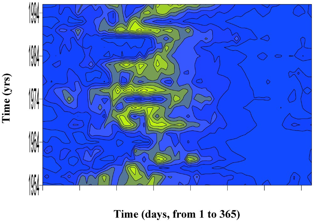
French Guiana main river discharges (Maroni River at the Langata–Biki station) as a function of time along the x- and y-axis. The x-axis represents a short time scale (sampling time: days), while the y-axis shows a long one (chosen periodicity: one year). A grey scale combined with an exact 2D polynomial interpolation (slightly smoothed here) allows easy visualisation of discharge variations (in m3 s−1). Intensity and interannual trends of low (dark) and high (light) water seasons are easily observed over the recorded period 1954–1996.
Courbe de débit du principal fleuve de Guyane française (Le Maroni, mesuré à la station Langata–Biki) en fonction du temps, selon les axes x et y. L'axe x possède une haute résolution temporelle (celle de l'échantillonnage : le jour), tandis que l'axe y a une basse résolution temporelle (la périodicité annuelle). Une échelle en niveaux de gris, combinée à une interpolation polynomiale 2D exacte, permet une meilleure visualisation des variations de débits (en m3 s−1). Les intensités et tendances interannuelles des saisons d'étiage et de crue sont facilement visibles sur la période mesurée (1954–1996).
La propriété la plus pertinente du DXM pour cette étude est sa capacité à identifier les ressemblances multi-temporelles entre les processus hydroclimatiques synthétisés par l'indice SOI et des débits de Guyane française (Fig. 2a et b). Leurs deux cartes respectives montrent en effet d'étonnantes similitudes, qui peuvent être quantifiées grâce à un coefficient « étendu » de corrélation croisée (ECC) conçu sur la même formulation mathématique que la CCF (équation (1)). Ce coefficient étendu de corrélation croisée intègre les coefficients de corrélation croisée entre un pixel de la première image et les pixels voisins de son homologue dans la seconde, au sein d'une fenêtre de calcul glissant sur les images. Ces zones peuvent être carrées ou rectangulaires et nous avons optimisé leur taille de ±2 à ±5 pixels autour du pixel central de calcul pour la périodicité annuelle (axe des y). Après une moyenne des coefficients de chaque pixel et des fenêtres de calcul variables, on obtient l'équivalent d'un facteur de ressemblance entre les deux images, qui peut reproduire une CCF par le décalage progressif de la série temporelle au sein de la seconde image. Les tests avec des paramètres de signaux différents ont toujours montré que la technique DXM est au moins aussi performante que l'analyse de Fourier pour détecter une influence étendue (avec des niveaux de confiance souvent supérieurs à 99 %). Nous avons estimé les niveaux de confiance (CL) par simulations Monte Carlo, à ECC∼0,13 et ∼0,16±5 % pour les seuils respectifs de 95 et 99 %.
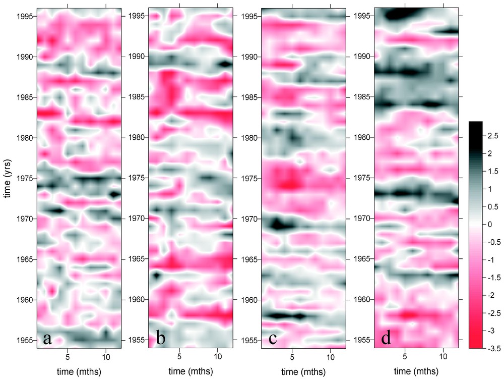
SOI (a), French Guiana discharges (b), South Atlantic SSTA (c) and North Atlantic SSTA (d) DXM with 12-month imposed period maps. Monthly index values are plotted as a function of time along the x- and y-axes. The x-axis represents a short time scale (the sampling time), while the y-axis shows a long one (the chosen periodicity). A common colour scale combined with an exact 2D polynomial interpolation makes it easy to visualise index variations depending on how the DXM is ‘read’. Intensity and interannual trends of El Niño (in red) and La Niña (in black) events, of discharges (floods in black) and Atlantic temperature anomalies (positive in black) are easily observed over the period 1950–1999.
Cartes DXM, avec une périodicité annuelle, du SOI (a), des débits guyanais (b), des SSTA de l'Atlantique sud (c) et nord (d). Les valeurs mensuelles standardisées de ces indices hydroclimatiques sont présentées en fonction du temps selon les axes x et y. L'axe x possède une haute résolution temporelle (le mois), tandis que l'axe y a une basse résolution temporelle (la périodicité annuelle). Une échelle de couleur commune, combinée à une interpolation polynomiale 2D exacte, permet une meilleure visualisation des variations d'indices, selon le sens de lecture. Les intensités et tendances interannuelles des événements El Niño (en rouge) et La Niña (en noir), des débits (crues en noir) et des anomalies de températures de surface de l'Atlantique (positives en noir) sont facilement visibles sur la période mesurée (1954–1996).
4 Résultats
La courbe (spectre en puissance) ECC de la comparaison SOI/débits présente une forme différente de celle CCF classique (Fig. 4a). Le maximum principal au décalage ∼5 mois a été légèrement décalé et réduit d'environ 9 %, avec un niveau de confiance accru (supérieur à 99 %). Un second maximum apparaı̂t au décalage de 18 mois, tandis qu'il restait négligeable avec la CCF. Une corrélation quasi instantanée d'ENSO avec la pluviométrie et les débits de Guyane semble combinée à une autre corrélation, plus retardée et opposée. La prise en compte d'une possible influence étendue a clairement réduit l'amplitude de la première au profit de la seconde. Ainsi, dans l'hypothèse où ces corrélations traduisent des influences, ce ne serait pas seulement l'événement La Niña qui favoriserait une augmentation de la pluviométrie en Guyane, mais aussi l'événement El Niño, qui a eu lieu environ deux ans auparavant. Cette constatation est confirmée dans les faits, la combinaison des deux phénomènes au cours de la période 1954–1996 occasionnant une augmentation (respectivement réduction) des débits d'environ +10 (respectivement −8 %). On pourrait être tenté d'attribuer une variation des débits à la seule phase récente d'ENSO, du fait de l'alternance presque régulière de phases opposées dans ce phénomène. Mais si notre analyse est exacte, on doit, par exemple, pouvoir trouver une forte augmentation des débits de Guyane environ deux ans après un événement El Niño, même sans événement La Niña récent. C'est exactement ce qui s'est produit au cours de l'année 2000, où la Guyane a probablement enregistré les plus importantes inondations du XXe siècle, juste deux ans après l'événement El Niño, probablement le plus intense de la même période. Notons que ces années récentes n'ont pas été inclues dans notre précédente analyse, qui s'étend jusqu'en 1996, et n'ont donc pas pu contribuer à cette conclusion.
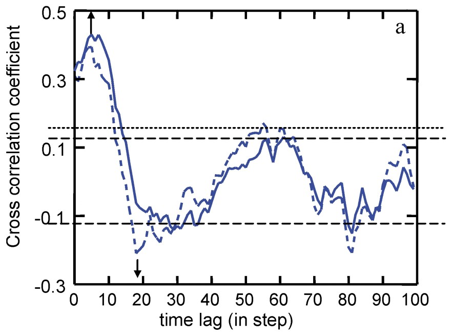
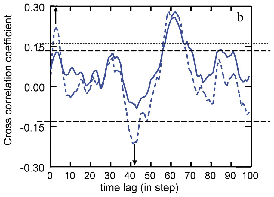
SOI/streamflows (a) and SA/streamflows (b) cross-correlation plots. Classical CCF (continuous line) and ECC (dashed line) are plotted as a function of positive time lags (in months). Considering long-lasting processes modifies and often accentuates the cross-correlation coefficient extremums. The 95 and 99% CL for ECC curves are shown.
Courbes de corrélation des couples SOI/débits (a) et SA/débits (b). Les corrélations ECC (trait pointillé) et CCF (trait continu) sont dessinées en fonction du décalage temporel (en mois) des signaux du couple étudié. Considérer ces signaux étendus dans la durée modifie, et souvent accentue, les extremums du coefficient de corrélation croisée. Les niveaux de confiance à 95 et 99% des courbes ECC sont reportés.
Il ne fait pas de doute que, par sa proximité, l'océan Atlantique influence également les débits de Guyane. Nous avons ainsi estimé les ECC des couples NA/débits et SA/débits, qui ont montré des influences instantanées respectives de ECC=−0,211 et 0,221±0,008 (à des décalages de 3 et 4 mois) et à des niveaux de confiance supérieurs à 99 % (Fig. 4(b), NA ECC non montré). L'extremum du spectre lié à l'océan Atlantique sud en particulier a ainsi été rehaussé de plus de 40 %, traduisant le fait que, statistiquement, l'augmentation des débits de Guyane est corrélée avec une température de surface positive dans l'Atlantique nord et négative dans l'Atlantique sud trois mois plus tard. Cette alternance, causée par les connexions atmosphériques entre ces trois zones, n'avait pas été clairement identifiée auparavant, du fait de l'apparente nature décorrélée de l'océan Atlantique sud avec ses régions voisines. Un second extremum significatif dans ces courbes ECC est visible autour du décalage de ∼40 mois (ECC=−0,32 et −0,22±0,01 pour les influences respectives de NA et SA, supérieurs à 99 % de CL). Là encore, l'accroissement du second pic lié à SA est un nouvel indice fort en faveur de l'existence d'une corrélation retardée et combinée des différentes parties de l'Atlantique avec les débits de Guyane française. Les différences importantes révélées entre les CCF et les ECC, incluant SA, trahissent un comportement complexe et étendu dans le temps du Sud de l'Atlantique et méritent d'être étudiées plus en détail (à ce stade, nous ne disposions pas des données et modèles nécessaires).
5 Conclusion
Le choix de prendre en compte les processus climatiques avec une influence étendue dans le temps nous a permis de mettre à jour de nouvelles corrélations retardées entre ENSO, l'océan Atlantique et les débits des fleuves de Guyane française. Les corrélations mises en évidence sont par ailleurs conformes à celles quasi instantanées, déjà connues. Cette hypothèse de travail présente l'intérêt de proposer une interprétation originale aux pluies catastrophiques de l'an 2000 qui ont été enregistrées en Guyane (et ailleurs), comme étant éventuellement la conséquence retardée de l'événement El Niño de 1997–1998, plus que celle de l'événement La Niña de 1999. Ces constations nous incitent à étudier à l'avenir, plus en détail, cet effet d'extension dans le temps des phénomènes hydroclimatiques.
1 Introduction
The El Niño/Southern Oscillation (ENSO) phenomenon is generally characterised by its Southern Oscillation Index (SOI) and produces interannual variations in the atmospheric circulation and the hydrological cycle [20,25]. It causes regional, sometimes devastating, climatic effects outside the tropics by shifting the normal precipitation and temperature patterns [6,22]. South America in particular, due to its proximity to the ENSO core region, has been strongly affected for thousands of years [21]. It has been explained how, through atmospheric teleconnections, ENSO events affect South America and the Atlantic Basin [1]. The disturbances generated by an El Niño event are summarised as two main processes. First, a westward shift of the convection zone, normally centred on Amazonia, is associated with the convergence of easterly and westerly winds [28]. Atlantic trade winds are enhanced by this closer convergence zone and activate the small Atlantic atmospheric cell (sometimes called the ‘Atlantic Walker cell’). Second, this configuration is favoured by a blocking situation of polar frontal systems in a zone extending from southern Peru to southern Brazil and related to a stronger subtropical jetstream [14]. The results of these conditions are abnormally high rainfall rates in the blocking zone and drought in the regions located northward, i.e., Northeast Brazil and Guiana [12].
In the year following a significant El Niño event, the tropical North Atlantic (NA) is often characterised by unusually warm Sea Surface Temperature Anomalies (SSTA), while the tropical South tropical Atlantic (SA) sometimes, but not always, behaves in the opposite fashion [7]. Nowadays, the ENSO phenomenon seems to be the main cause of the ‘dipole’ structure correlating tropical Atlantic SST and rainfall in northeastern Brazil [23]. During La Niña events, the subsidence part of the equatorial Atlantic Walker cell becomes weaker and tends to diverge. This reduces Atlantic trade winds and pushes the Inter-Tropical Convergence Zone southward, which produces increased precipitation in northeastern Brazil and Guiana.
As an illustration of these mechanisms, we computed the Cross-Correlation Function (CCF) between SOI and French Guiana streamflows and found quite a high correlation with a 5-month time lag. By making this calculation we made the (strong?) simplifying assumption that a precise date of an El Niño event directly generates a decrease in French Guiana rainfalls at another isolated moment. To determine the value of this assumption, we propose here a new approach based on simple statistical arguments. Note that we deal here with associations, not causalities; nevertheless, they provide significant clues to the way the processes influence each other.
2 Data and scientific context
Few studies of the hydrology of the Guiana plateau are available [11]. Our data come from French Guiana, a French overseas administrative region located on the Atlantic coast north of Brazil, with an approximate surface area of 84 000 km2. We took the mean monthly discharge of its two main rivers, the Maroni and Oyapock (measurement accuracy assumed to be ∼5%) recorded by the ‘Institut de recherche pour le développement’ (IRD, formerly ORSTOM) over the period January 1954 to December 1996. Both time series have been standardised, averaged and deseasonalised (by normalisation with the 42-year average). We then compared (thanks to the NOAA/CPC website: http://www.cpc.ncep.noaa.gov/data/indices/) the French Guiana streamflows with the corresponding monthly SOI, NA and SA indices. The SOI/streamflows comparison clearly shows a maximum cross-correlation of 0.47±0.05 at a ∼5-months time lag. This peak is much higher than the 95% confidence level (CL). It confirms that statistically, during the last half century, an El Niño (La Niña) event is followed by decreasing (increasing) discharge approximately 6 months later in French Guiana.
Weaker relationships were found with the NA and SA indices: −0.183 and 0.128±0.008, with respectively 4- and 3-month delays, still above the 95% CL. Negative precipitation (and then discharge) anomalies in French Guiana tend to correspond to warm events in the tropical Pacific, cold SSTA in the western North Atlantic and sometimes (only) warm SSTA in the western South Atlantic. In the year immediately following La Niña (respectively El Niño) events, the French Guiana discharges show an average increase of +8% (respectively −7%). The maximum discharge increase over the past half-century was found in 1989 with +59% compared to the annual mean, while the maximum decrease was observed in 1983 with −51%.
Here, the classical CCF gives the correlation coefficients between the two curves on a month-by-month basis. This assumes that an isolated portion at a given month of an El Niño event directly generates a decrease in French Guiana rainfall at another precise month, 5 to 6 months later. But such large climate phenomena have inertia and may be a ‘memory’ [13,17]. Therefore, there is an intrinsic consistent pattern between the successive steps of a process like El Niño, but also these steps are likely to simultaneously influence neighbouring processes. This consistency has already been examined, for instance, with the delayed oscillator concept [27], as well as with that of delayed influences [18,29]. Moreover, even in these studies, processes are compared date-by-date. However, what is called an El Niño impact is not the influence of a unique negative SOI value, but the integration of the influence of the negative index values between the last and the next positive ones. Hence, to better explore the cross-correlation between such extended physical phenomena, we imagined a new tool able to simultaneously visualise and quantify the correlation at different time scales and resolutions.
While many methods are able to examine physical processes that occur over a range of time scales [10,19], few can quantify scaling relations between processes. The most commonly used concept with this property is the Fourier (and Wavelet) covariance [3,8]. However, these methods are particularly well suited for long time series and highly periodical phenomena, but they are quite ineffective for short quasi-periodical signals such as hydrological or climate indices. Furthermore, scientists usually consider that lags between two signals are independent of time scale and resolution [9,26]. Recent time–frequency approaches have also been used to detect irregular multi-scale variations of real processes [4,5,24] (and references therein), but as opposed to the covariance methods, they are time consuming or inefficient for quantifying scaling relations between processes.
3 New methodology
When studying coupled processes, scientists usually consider that each step of the first process influences another unique step in the second process. Our first hypothesis is that neglecting a probable ‘extended influence’ modifies the final result. By computing the cross-correlation between two signal dates with a constant time lag, a classical CCF has the effect of averaging the different time scale influences and hence of hiding information on the coupling mechanism.
The extended influence hypothesis proposes to compute cross-correlation coefficients between successive steps and successive periods at the same time step. This can be achieved with the help of a new method, called the Digital X Model (DXM, X for the studied index or parameter). We used the spatial dimensions in order to visualise the temporal one, and plotted a dataset (for instance, the Maroni daily streamflows) as a function of two temporal axes with different time resolutions: the sampling time (one day) along the x-axis and a chosen periodicity (one year) along the y-axis (Fig. 1). The Maroni floods (light) or low waters (dark) are clearly visible on its DXM map, during the 1954–1996 period. For ease of viewing (but not for calculation), the DXM values (or ‘the X values of the DXM’) are interpolated with exact 2D polynomial functions and visualised with a colour scale. Hence, the intra- and inter-annual discharge variations are instantaneously recognisable. Note that interpolating this map (or image, composed of pixels) is equivalent to making the hypothesis that the X parameter is a continuous field along the x- and y-axes, whereas it could be a discrete one. Hence, our second and last hypothesis is that each discrete temporal signal can be considered as a continuous field in our multi-temporal analysis. The interpolated values along the y-axis have no reality, but the trend of the successive steps has a real significance and represents the probable value ‘between’ the two successive y periods. Others interesting DXM properties are not discussed here (work in progress).
What is relevant in our context is the ability of the DXM method to visually and computationally identify resemblance between processes such as the temporal variations of SOI and French Guiana discharges (Fig. 2a and b). The two maps show astonishing similarities. South and North Atlantic SSTA (Fig. 2c and d) are shown for information. To quantify these multitemporal similarities, we developed an ‘Extended’ Cross-Correlation (ECC) coefficient with a similar mathematical definition than the cross-correlation coefficient. For two images I1 and I2 plotted with the same imposed periodicity (or y-axis sampling), we combined the cross-correlation coefficients involving the central pixel of the first image pi,j|I1 and a specific neighbouring position of the second image pi+u,j+v|I2, within a small window calculation:
| (1) |
We tested and validated the DXM/ECC method with fully controlled simulated signals. To reproduce plausible hydro-climatic curves, the simulated signals were constructed as follows:
- (i) a 500-point white noise signal was synthesised;
- (ii) a second influenced signal was built by translating, summing or multiplying (with a 1/k attenuation factor, k=20 steps) the successive values of the first signal, always keeping this first signal indices (the causes) lower than the second signal indices (the consequence).
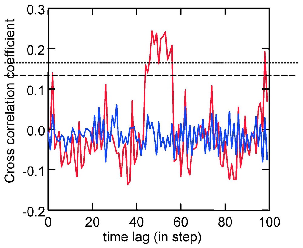
CCF/ECC plot comparison for simulated signals. If the signal y is constructed with a weighted (1/k) product of successive and periodically successive x values shifted by 50 steps to simulate an attenuated influence of x on y, the ECC technique (solid line) is much more efficient than the CCF one (dashed line) to uncover this correlation. 95 and 99% CL for the ECC curve are shown.
Comparaison de courbes CCF et ECC pour des signaux simulés. La méthode ECC (en rouge) se révèle bien plus efficace que celle CCF (en bleu) pour détecter une corrélation entre un signal et son homologue bruité et décalé de 50 pas, construit comme le produit atténué (d'un poids 1/k) d'un signal périodique à deux échelles temporelles différentes. Les niveaux de confiance à 95 et 99% de la courbe ECC sont reportés.
4 Results
The SOI/streamflows ECC plot exhibits a different shape than the classical CCF plot (Fig. 4a). The main extremum at a 5-month time lag has been reduced (by ∼−9% at ECC=0.393±0.009, much higher than the 99% CL) and slightly shifted. A second extremum appears with a 18-month time lag (ECC=−0.21±0.01), while it was absent or negligible in the CCF plot (relatively to the CCF CL). This extremum confirms the existence of both an almost instantaneous and a delayed correlation between the ENSO phenomenon and the French Guiana discharges. Considering the long-lasting effect of these climatic phenomena, the correlation with the short time lag has clearly been reduced, while the correlation with a long time lag has been increased. One can therefore say that not only is a La Niña event linked to an increase in French Guiana discharges, but also that an El Niño event seems to increase, about two years later, these discharges. The ECC analysis of French Guiana discharges indicates that the direct effect of a La Niña event combined with the delayed effect of an El Niño event that occurred two years earlier increases the discharges, on average between 1954 and 1996, by 25%; this increase is only of 10% in case of a La Niña event alone, and of 8% in case of a delayed El Niño event alone.
As ENSO phases alternate quite regularly, the delayed correlation could be statistically attributed to the presence of the opposite phase. But if our results are statistically true, we should be able to find increasing discharges about two years after a Niño event, without a pronounced (even if present) La Niña event the year before. As an example, this was exactly the case in year 2000, when French Guiana had the heaviest floods in the past century, two years after the most intense El Niño of the past decades, and during a weak La Niña event. Note that the last years were not included in our dataset, which ends in 1996, and the 2000 event did not contribute to this conclusion.
While the ENSO correlation with the French Guiana streamflows seems to be the most important one, there is no doubt that the Atlantic Ocean, by its proximity, also contributes to these time curves. This is why we examined the NA/streamflows (respectively SA/streamflows) ECC plots over the same period (Figs. 2c and 4b). In both curves, we found an obvious almost instantaneous correlation at a 3-month time lag with an ECC=−0.211±0.008 (respectively at 4-month time lag and ECC=0.221±0.008) higher than 99% CL (Fig. 4b, NA ECC is not shown). The first SA/streamflow extremum, in particular, was not obvious on the CCF, before we considered the possible lasting influence of this part of the Atlantic Ocean (∼42% of peak intensity increase). This means that statistically, increasing discharge in French Guiana is correlated with positive SSTA in the tropical North Atlantic and negative SSTA in the tropical South Atlantic, approximately three months later. This reverse mechanism is based on atmospheric connections between the North and South Atlantic Basins and adjacent continental areas [16]. A real swing appears between Atlantic conditions and the French Guiana discharges. This swinging instantaneous link (and possibly influence) had not been clearly identified up to now, because of the apparent lack of correlation between the SA SSTA and neighbouring processes.
A second significant common extremum is also visible in both ECC curves at ∼40-month time lag: ECC=−0.32±0.01 for the NA influence (respectively −0.22±0.01 for the SA influence), still higher than the 99% CL. The SA/streamflow extremum has again significantly increased by ∼62%. Hence, the North and South Atlantic should be in phase over the long term and correlated with the French Guiana climate. This is confirmed by the NA/SA ECC plot (not shown). As mentioned in the previous section, the difference between the SA/streamflows CCF and ECC suggests that the South Atlantic part behaves with complex and long-lasting processes. At this stage, we do not have enough information to explain the SA behaviour and influence on South America.
5 Conclusion
By considering long-lasting physical processes, we discovered new extended correlations between ENSO, the South Atlantic fluctuations, and French Guiana discharges. Hence, the well-known irregularities and impacts of the ENSO phenomenon could be attributed not only to an intrinsic chaotic behaviour or seasonal variations, but also to the inertia of the involved climatic phenomena. Interestingly, our hypothesis of extended influence could explain the numerous disasters of the year 2000 as the impact of the strong (delayed) 1997–1998 El Niño event. These observations led us to understand and model the ENSO effect with an intrinsic consistency and an extended influence at different time lags, as is presently done in the spatial domain by some hierarchical models [15].