

Version française abrégée
1 Introduction
L'estimation des contraintes horizontales dans un forage vertical à l'aide de diagraphies dipolaires soniques nécessite l'analyse de l'anisotropie des ondes de cisaillement [2,5,6,8,10,11,14]. Une manière d'estimer les paramètres de la relation vitesse-contrainte [7,13] consiste à modifier la pression du fluide du puits, de façon à influencer les courbes de dispersion des ondes flexurales [9,12]. Des diagraphies dipolaires soniques ont été acquises dans le puits AIG 10 entre les profondeurs 711 et 1004 m, dans les carbonates compacts, en trois passages successifs pour lesquels les pressions du fluide du puits ont été modifiées (0.1, 2.3, et 3.0 MPa). Dans cet article, nous présentons l'étude de l'anisotropie azimutale des ondes S, déduite d'une méthode de rotation 4-composantes [1,2] et de l'analyse des courbes de dispersion des ondes flexurales, ainsi qu'une première interprétation de l'anisotropie observée.
2 Analyse des diagraphies dipolaires soniques
Les diagraphies dipolaires soniques du puits AIG 10 ont été acquises avec l'outil DSI∗ de Schlumberger [3]. Pour chaque profondeur, les quatre formes d'ondes acquises sur une paire de récepteurs orthogonaux, associée à une paire de sources orthogonales, sont soumises à une rotation Alford [1,2], qui calcule la direction de l'onde S rapide lorsque la formation est de nature transverse isotrope, avec un axe de symétrie orthogonal à l'axe du puits. L'angle mesuré est celui qui minimise l'énergie des deux composantes croisées. Les formes d'onde sont alors orientées en fonction de la direction de l'onde S rapide et soumises à un traitement de similitude, de manière à obtenir les lenteurs des ondes S rapides et lentes [2,4]. Dans un milieu isotrope, les formes d'onde rapide et lente se superposent alors que dans un milieu anisotrope, les formes d'onde rapide arrivent en premier. En complément, l'analyse des courbes de dispersion des ondes flexurales révèle la présence d'anisotropie lorsque les courbes de dispersion de deux récepteurs orthogonaux se séparent dans le domaine basse-fréquence [6,8,13,14]. Les diagraphies dipolaires soniques sont présentées pour les profondeurs 720–855 m (Fig. 1). L'anisotropie est identifiée à l'aide d'une combinaison de facteurs : fort signal sur bruit, faible minimum et large maximum d'énergie dans la rotation Alford, stabilité et faible incertitude de l'azimut de l'onde S rapide, et une claire séparation des courbes de dispersion, des temps d'arrivée et des lenteurs entre les directions des ondes rapides et lentes. Dans l'intervalle de profondeur 701–1004 m, nous avons sélectionné quatre zones d'intérêt A (735–753 m), B (753–773 m), C (779–785 m), et D (809–850 m). Ces sections spécifiques du puits montrent des caractéristiques évidentes, soit d'anisotropie azimutale d'intensité moyenne à large (9–25 %), en dessous de la faille d'Aigion, par exemple, pour les intervalles 779–784 (zone C, Fig. 1) et 809–816 m (zone D, Figs. 1 et 3), avec une onde S rapide selon l'azimut 105°, soit de milieu homogène isotrope (zone A, 735–753 m, Fig. 2) entre l'extrémité du tubage et la faille. La présence de la faille coı̈ncide avec l'identification de vitesses lentes sur un intervalle approximatif de 12–14 m (zone B, Fig. 1). L'analyse des données révèle que la formation n'est pas sensible d'un point de vue acoustique à une différence de pression appliquée de 3 MPa.
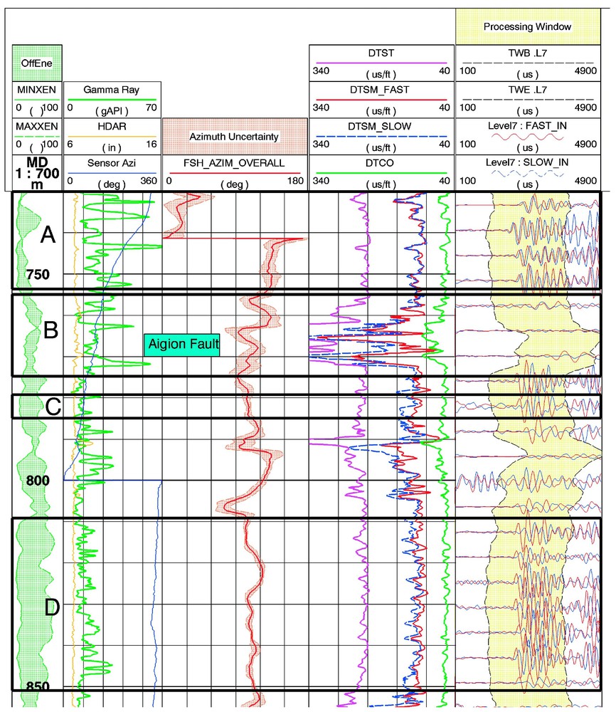
Dipole sonic logs for the AIG 10 well for depth interval 730–855 m. In the depth track, the green shaded area is bounded by the curves of the minimum and maximum energies in the cross components. The second track contains gamma ray (green line), average borehole diameter (yellow line), and the sensor azimuth from the GPIT (blue line). The next three tracks show, respectively, the fast-shear direction with uncertainty, the slowness logs (Stoneley, compressional, fast-shear, and slow-shear), and the rotated waveforms with the processing window used to obtain the shear slowness. Zones A, B, C, and D are the four zones of interest interpreted in text.
Diagraphies soniques dipolaires pour le puits AIG 10, à la profondeur de 730–855 m. Dans le tracé de profondeur, la zone verte ombrée est limitée par les courbes d'énergie minimum et maximum des composantes croisées. Le deuxième tracé comporte le rayonnement gamma (ligne verte), le diamètre moyen de forage (ligne jaune) et l'azimut du capteur GPIT (ligne bleue). Les trois tracés suivants représentent respectivement la direction de cisaillement rapide avec incertitude, les diagraphies de lenteurs (Stonely, en compressions, cisaillement rapide et cisaillement lent) et les formes d'onde après rotation avec la fenêtre de traitement utilisée pour obtenir les lenteurs de cisaillement. Les zones A, B, C, et D sont les quatre zones intéressantes, interprétées dans le texte.
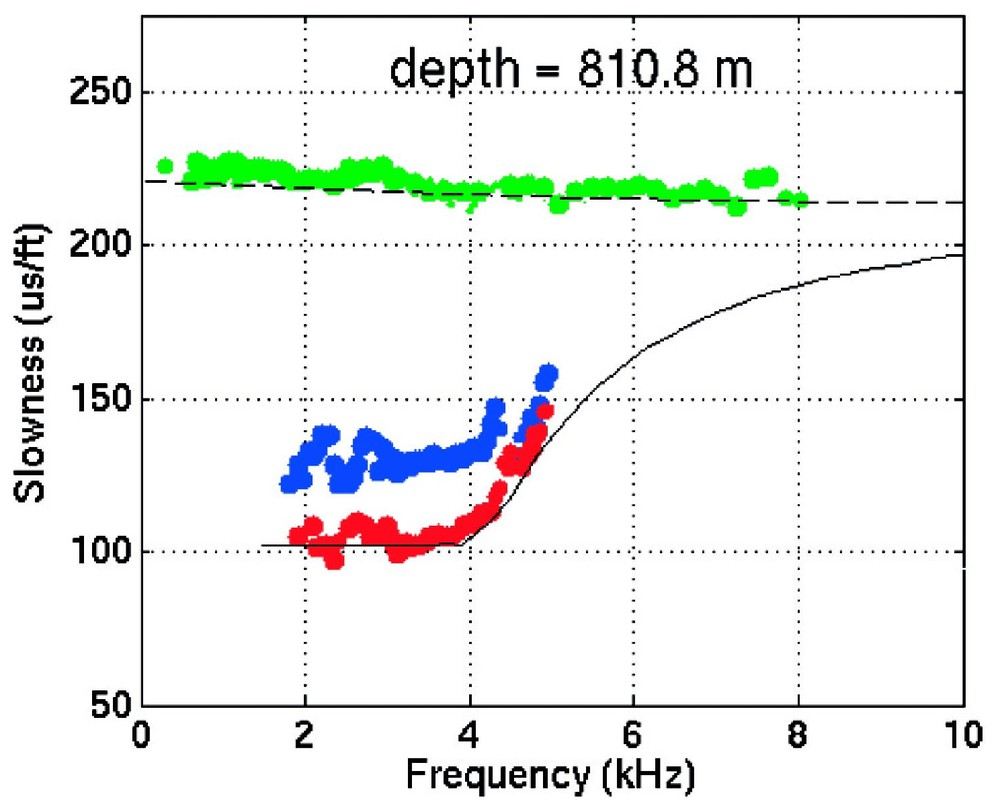
Slowness dispersion curves at depth 810.8 m in the AIG 10 well. The two orthogonal flexural modes (XX in red and YY in blue) are displayed with the monopole Stoneley (green). The solid and dashed black lines are the same as in Fig. 2. The two shear slownesses at low frequency (2–4 kHz) are clearly separated and indicate the presence of strong azimuthal anisotropy (∼25%).
Courbes de dispersion de lenteur à la profondeur de 810,8 m dans le puits AIG 10. Les deux modes flexuraux orthogonaux (XX en rouge et YY en bleu) sont représentés avec le monopole Stoneley (en vert). Les lignes noires continues et en tiretés sont les mêmes que pour la Fig. 2. Les deux lenteurs de cisaillement à basse fréquence (2–4 kHz) sont nettement séparées et indiquent la présence d'une forte anisotropie azimutale (∼25%).
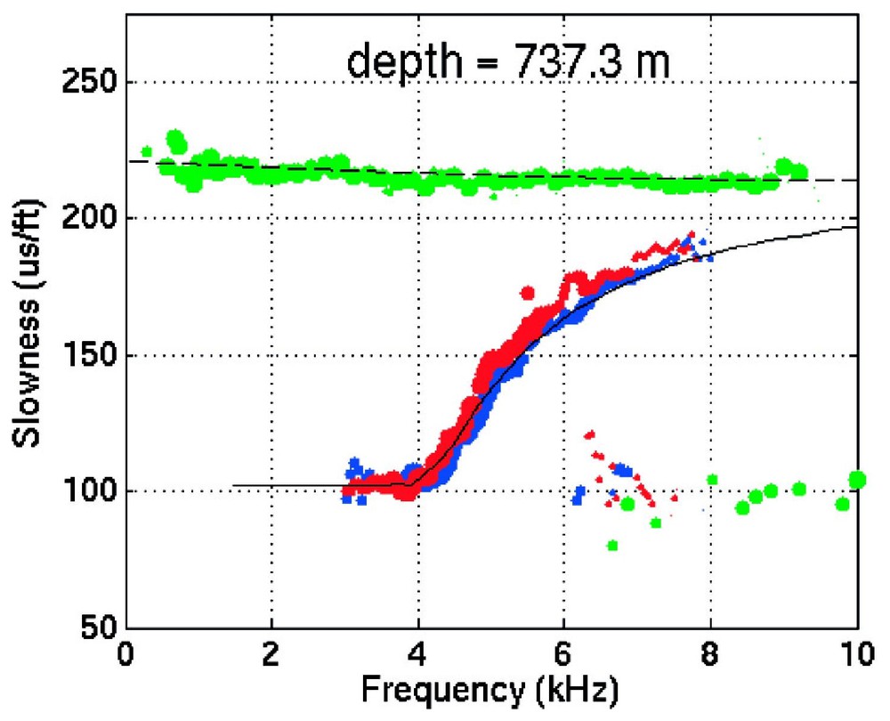
Slowness dispersion curves at depth 737.3 m in the AIG 10 well. The two orthogonal flexural modes (XX in red and YY in blue) are displayed with the monopole Stoneley (green). The solid and dashed black lines are the results of theoretical calculations for a homogeneous isotropic formation (50 and 102 μs/ft for respectively P- and S-wave slowness; a fast formation) and for a pure monopole and dipole source (20.32 cm diameter circular borehole with a mud slowness of 210 μs/ft). The dispersion curves clearly match a homogeneous isotropic model at this depth.
Courbes de dispersion de lenteur à la profondeur de 737,3 m dans le puits AIG 10. Les deux modes flexuraux orthogonaux (XX en rouge et YY en bleu) sont représentés avec le monopole Stoneley (en vert). Les lignes noires continues et en tiretés sont le résultat de calculs théoriques pour une formation isotrope homogène (50 et 102 μs/ft pour la lenteur des ondes P et celle des ondes S respectivement ; formation rapide) et pour une source pure monopolaire et dipolaire (20,32 cm de diamètre, avec une vitesse de la boue de 210 μs/ft). Les courbes de dispersion indiquent clairement un modèle isotrope homogène à cette profondeur.
3 Interprétation et conclusions
Une anisotropie azimutale a été clairement observée en dessous de la faille d'Aigion dans les zones C et D, avec une direction de l'onde rapide principalement de 105°. Dans ces zones, les courbes de dispersion montrent des caractéristiques similaires indicatrices d'anisotropie intrinsèque ou induite par les contraintes pour les fréquences 1–4 kHz, mais ne permettent pas de choisir entre les mécanismes à l'origine de l'anisotropie, du fait de l'absence de signal au-delà de 5 kHz. En dépit de l'absence de variation des courbes de dispersion et de l'azimut de l'onde S rapide en fonction de la pression appliquée, nous observons une excellente répétabilité des mesures sur les trois diagraphies, indiquant les mêmes azimuts et lenteurs. Ces observations indiquent que les roches ne sont pas acoustiquement sensibles aux niveaux de pressions appliquées, mais n'indiquent pas que la contrainte différentielle horizontale est nulle. Cette faible sensibilité acoustique aux contraintes montrent que, si une anisotropie azimutale induite par les contraintes était observée, la différence entre les contraintes horizontales minimum et maximum devrait être grande.
Lorsque l'anisotropie est d'origine intrinsèque, des signatures structurales typiques sont généralement observées sur les diagraphies de résistivité (outil ). Les images de résistivité (Fig. 4) montrent que l'azimut des alternances sédimentaires et des fractures, respectivement 120° et 110°, est parallèle à la direction de l'onde S rapide dans la zone d'anisotropie (zone D), alors que cet azimut est orienté 170° pour la zone A d'isotropie, c'est-à-dire à environ 65° de l'azimut de l'onde S rapide des zones anisotropes. Ainsi, l'interprétation des données soniques en complément des diagraphies d'imageries suggère que l'anisotropie soit liée à la stratification et la présence de fractures et que la direction de l'onde de cisaillement rapide 105° soit cohérente avec la contrainte maximale horizontale régionale.
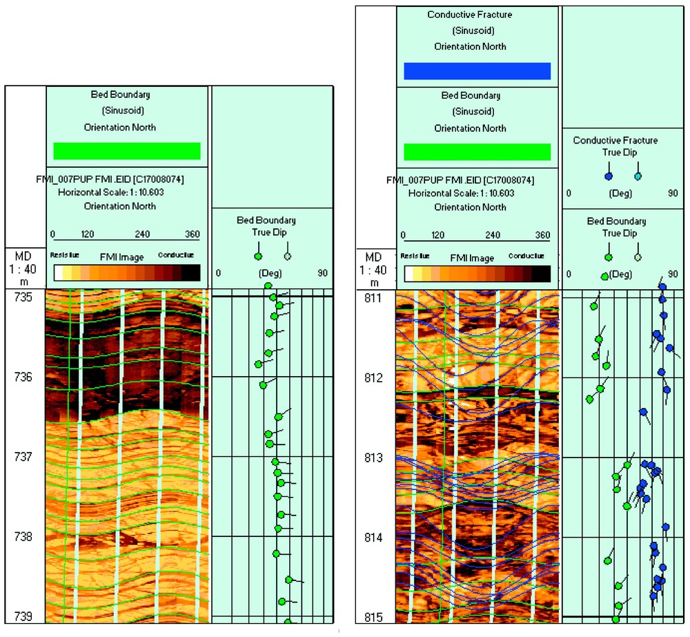
Resistivity image logs (FMI) for depths 735–739 m (zone A) and 811–815 m (zone D). Bed boundary (green) and conductive fracture (blue) sinusoids are presented with their associated dip and dip direction.
Diagraphies d'imagerie de résistivité (FMI) pour les profondeurs 735–739 m (zone A) et 811–815 m (zone B). Les sinusoı̈des de limite de banc (en vert) et de fracture conductrice (en bleu) sont présentées avec leurs pendage et direction de pendage associés.
1 Introduction
The estimation of the differential horizontal stresses in vertical boreholes using a sonic logging tool requires the measurement of both the shear velocities in stress-induced anisotropic formation and the acoustic stress sensitivity of the formation [8,10,13]. Dipole sonic logging tools provide the capability to measure shear in both fast and slow formations as well as to characterize the shear anisotropy of the formation [2,5]. Acoustic anisotropy can be either intrinsic (i.e., bedding, shales, aligned fractures) or stress-induced. Advanced frequency domain processing has shown that borehole flexural dispersion curves yield information to discriminate between different sources of anisotropy [6,8,11]. Alternative methods to distinguish intrinsic anisotropy from stress-induced anisotropy use information that may come from ultrasonic or resistivity borehole imaging logs. When stress causes the anisotropy, the acoustic stress-sensitivities of the formation are then required to calibrate the stress-velocity relationship [7,13]. A way to estimate the formation of stress sensitivity is to use changes in the pressure of the borehole fluid that are known to influence flexural dispersion curves [9,12]. Within the Corinth Rift Lab and the Aigion well (AIG 10), we attempted to estimate differential horizontal stresses by finding formation acoustic stress sensitivity by pressurizing the borehole and recording four-component flexural data.
Daniel et al. (this issue) report on the detailed structural analysis of these polydeformed carbonate rocks observed in the well. They describe both the pre-existing tectonic fabrics and the faults and fractures related to recent extension of the Aigion fault.
In this paper, we present sonic data acquired in the AIG 10 well using a dipole sonic logging tool between depths 711 m and 1004 m (depths are hereafter understood as meters below blow out preventer). Logging passes were done at three different applied borehole fluid pressures (0.1, 2.3, and 3.0 MPa). We first analyse the shear azimuthal anisotropy using the four-component rotation concept [1,2] and the analysis of dispersion curves [6] to assess the correct fast-shear direction and the amount of anisotropy. Next, we discuss the presence or absence of shear anisotropy and the repeatability of independent log measurements at different applied borehole fluid pressures.
2 Cross-dipole logging
The cross-dipole logs in the AIG 10 well were acquired using the Schlumberger (Dipole Shear Sonic Imager) tool. The DSI is a multireceiver tool [3] with a linear array of eight receiver stations (15.24 cm spacing), a monopole transmitter, and two orthogonal dipole transmitters (dipole source spacing is 15.24 cm, and the upper dipole transmitter is 3.35 m away from the nearest receiver). At each receiver station is a pair of orthogonal dipole receivers that form two arrays, each oriented in the direction of one of the dipole transmitters. Waveform data at each depth for anisotropy analysis are collected as four components: the output of the dipole receivers aligned (inline) and orthogonal (crossline) to each dipole transmitter [2]. The four sets of recorded waveforms are subjected to the so-called Alford rotation algorithm [1,2] that yields the fast shear direction with respect to a reference dipole source direction (the orientation of the tool is known using the ). The angle is the one at which the energy in the two cross-line components is minimized [2]. The maximum energy in the cross-components is also computed as an indicator of the fit of the waveforms to the Alford model, and a qualitative indicator of anisotropy magnitude. In an isotropic formation, both the maximum and minimum crossline energy will be small. For the case of a transverse isotropy (TI) where the borehole is perpendicular to the TI axis, the minimum crossline energy should be small and the maximum crossline energy becomes large, so that their difference is large (an example of a TI medium is a collection of horizontal beds where the TI symmetry axis is perpendicular to the beds). If the maximum is large but the minimum is not small, this observation implies that the formation anisotropy with respect to the borehole axis is either of a tilted transverse isotropy (TTI) or of lower anisotropy symmetry. The described technique is based on the following assumptions:
- (1) the medium is homogeneous for S-waves between sources and receiver array, and
- (2) the mechanical properties of the borehole wall are not altered.
The recorded waveforms are then rotated to the fast shear azimuth. The resulting fast- and slow-waveforms are then subjected to semblance processing for obtaining the fast- and slow-shear slownesses [2,4]. In an isotropic zone, the fast and slow waveforms are expected to overlay each other, whereas in an anisotropic zone, the fast waveform arrives earlier in time. In an anisotropic zone, the slownesses are separated.
In addition, dispersion curves provide a new analytical tool to study the waveforms in the frequency-slowness domain [6,13]. If the borehole axis is perpendicular to the TI axis, the two dispersion curves correspond to:
- (1) a slow shear direction where the dipole flexural mode is polarized parallel to the TI axis, and
- (2) a fast shear direction where the dipole flexural mode is polarized perpendicular to the TI axis.
3 Data analysis: The AIG 10 well
The cross-dipole logs for well AIG 10 are shown for depths 720–855 m (Fig. 1). The remaining parts of the log (701–720 m and 855–1004 m) are not displayed due to space limitations. In the depth track, the green shaded area is bounded by the curves of the minimum and maximum energies in the cross components, and gives an indication of the difference (OffEn) between the two curves. The second track contains gamma ray (green line), average borehole diameter (yellow line), and the transmitter azimuth from the (blue line). The next three tracks show, respectively, the fast-shear direction with uncertainty, the slowness logs (Stoneley, compressional, fast-shear, and slow-shear), and the rotated waveforms with the processing window used to obtain the fast azimuth. The fast shear azimuth was computed every 15.24 cm utilizing a sliding vertical processing window comprising 21 depth frames, here 3.05 m. Thus, the uncertainty on the direction is computed from the variation of azimuths over the 21 depth frames.
Finally, the anisotropy is identified using a combination of factors: strong signal, small minimum and large maximum energy in Alford rotation, arrival time difference, stable fast-shear azimuth, small uncertainty on azimuth, difference between slownesses, and clear separation of dispersion curves between fast- and slow-shear direction. In the depth interval 701–1004 m, we selected four zones for interpretation A (735–753 m), B (753–773 m), C (779–785 m), and D (809–850 m). The other sections of the logs (including section 850–1004 m, not presented here) have shown weak signal, unstable fast azimuth, large uncertainty, or absence of depth consistency on dispersion curves. Overall, the analysis of the data reveals an excellent repeatability of the measurements with no sensitivity to the level of applied borehole fluid pressure (0.1, 2.3, and 3.0 MPa).
3.1 Zone A (735–753 m)
The fast-azimuth analysis does not give any indication of clear azimuthal anisotropy from cross energy or stable direction (Fig. 1). The two flexural dispersion curves (red/blue) clearly coincide over the frequency interval 2–8 kHz (Fig. 2). These data are consistent with a homogeneous isotropic medium over a depth interval of approximately 18 m.
3.2 Zone B (753–773 m)
Analysis of logs images (J.-M. Daniel et al., this issue) has shown that the well crosses the Aigion Fault over depth interval 759–771 m. The presence of the fault coincides with lower velocities over an interval of approximately 12–14 m (Fig. 1).
3.3 Zone C (779–785 m)
The observed stable fast azimuth oriented 105° over a 5 m interval is supported by distinct slow and fast waveforms. The presence of moderate anisotropy (∼9% difference between fast- and slow-shear slownesses) is confirmed by two distinct parallel dispersion curves.
3.4 Zone D (809–850 m)
This section presents the best evidence of strong anisotropy with a stable fast azimuth oriented 105° over a 7 m interval, i.e., 809–816 m (Figs. 1 and 3). Fast and slow waveforms are associated with two distinct parallel dispersion curves at low frequencies (2–4 kHz) and reveal strong anisotropy in the order of approximately 25% (Fig. 3). Despite some small azimuth variations (105°–120°) consistent with the expected accuracy of the technique (i.e., ±5° at best), the rest of section D (i.e., 816–850 m) seems to exhibit the same anisotropic behaviour.
4 Discussion
Azimuthal anisotropy is clearly observed below the Aigion Fault in zones C (105° over ∼5 m), and D (105° over ∼7 m with its possible extension over the remaining of zone D with direction 105°–120° over ∼34 m) with an overall fast-shear direction mainly oriented 105°. Most of the observed dispersion curves in the anisotropic region exhibit the characteristic pattern as shown in Fig. 3: clearly separated curves in the frequency band 1–4 kHz, merging curves from 4–5 kHz, and absence of signal above 5 kHz. The dispersion curves extracted from data with borehole fluid pressure at 2.3 and 3.0 MPa show the same pattern with a slight extension of the high-frequency zone up to 5.5 kHz. For stiff formations similar to those encountered in this well (similar hole size), Sinha et al. [13] show that the dispersion curves will tend to be close above 4 kHz if intrinsic anisotropy is present. If the stress-induced mechanism is involved, the crossover between the two curves will occur around 6 kHz. Therefore, using only the AIG 10-well dispersion curves, it is difficult to discriminate without ambiguity the source of the anisotropy, as the highest frequency part of the signal was not excited.
We have not observed any change in the shear slowness when a fluid pressure of 3 MPa (the maximum safe pressure allowed) was applied. However, we have observed excellent tool repeatability with the three logs showing same azimuths and slownesses within the accuracy of the measurements. This means that the rock is not acoustically sensitive to the pressure levels applied, but does not imply that differential stress is absent. If stress-induced azimuthal anisotropy were present, we would expect large differences in the minimum and maximum horizontal stresses.
If the anisotropy were of intrinsic origin, we would expect to observe typical features on image logs, such as bedding or aligned fractures. For this purpose, we compare the resistivity image logs (FMI∗) of the isotropic zone A and the anisotropic zone D (Fig. 4). The borehole imagery (Fig. 4) between 735 and 739 m shows consistent bedding dipping about 40° to the east. Thin electrically conductive fractures, while fairly abundant, are typically bound by stratigraphic layering. While the borehole is fairly intact, both the FMI and the indicate mechanical damage on the borehole's western side. The borehole imagery between 811 and 815 m (zone D, Fig. 4) shows consistent bedding dipping about 25° to the north-northeast. Electrically conductive fractures appear wider, more continuous, and more abundant than in the shallower zone A. These fractures are dipping about 60–70° to the south. The borehole is intact and close to circular. Thus, the strike of the bedding and fractures, respectively 120° and 110°, in section D is almost parallel to the fast shear azimuth, 105°. However, in the isotropic zone A, the strike of bedding and fractures, 170°, is approximately 65° from the fast shear azimuth observed in the anisotropic zones of the borehole. The presence of significant bedding dip is consistent with non-zero minimum cross energy observed in the dipole anisotropy log. This observation implies that the formation anisotropy with respect to the borehole axis is that of a tilted transverse isotropy (TTI) or of lower anisotropy symmetry.
From the orientation of the Aigion Fault and earthquake focal mechanisms, the regional maximum horizontal stress direction is believed to have an approximate azimuth of 100–110°. It is possible that in section D, the alignment of the intrinsic anisotropy (bedding and fractures) with the regional maximum horizontal stress produces the observed sonic anisotropy with a fast shear orientation parallel to the intrinsic and stress induced anisotropy. In contrast, in the isotropic section A, the non-alignment of intrinsic anisotropy and stress-induced anisotropy produce a measurement with no apparent anisotropy. When the in situ stresses are known more precisely, these preliminary results can possibly be more accurately quantified.
5 Conclusions
Within the Corinth Rift Lab, we have attempted to estimate differential horizontal stresses by finding formation acoustic stress-sensitivity by pressurizing the borehole and recording four-component borehole flexural data. Using a new experimental design, dipole sonic data have been acquired in the AIG 10 well during three passes of a sonic logging tool at three different borehole fluid pressures (0.1, 2.3, and 3.0 MPa). We have analysed the shear azimuthal anisotropy to assess the fast-shear azimuth using the Alford rotation concept and characterize the anisotropy using the flexural dispersion curves. Specific sections of the well reveal clear characteristics of either moderate to large azimuthal anisotropy (9–25%) below the fault, e.g., 779–784 and 809–816 m, with a fast-shear azimuth directed 105°, or homogeneous isotropic medium (i.e., 735–753 m) between the casing shoe and the Aigion Fault. The presence of the fault is coincident with the identification of lower velocities over an interval of approximately 12–14 m. Analysis of the data reveals that the formation is not acoustically stress sensitive to the 3 MPa differential pressure applied, which prevents any quantitative stress estimation. However, excellent sonic log repeatability has been observed with the three passes. The interpretation of the sonic data with complementary image logs suggests the anisotropy is due to intrinsic fractures and bedding, and the fast-shear direction 105° is consistent with the regional maximum horizontal stress.
∗Mark of Schlumberger.
Acknowledgements
We would like to thank the European Union for support of the acquisition of the data under project ENK6-CT-2000–00056, and F.-H. Cornet (IPGP) who initiated and supported the collaboration leading to this work. We are grateful to U. Sperandio and G. Tumbiolo (Schlumberger Milan) for all their support in designing and planning the field experiment. We wish also to thank Jean-Marc Daniel (IFP) for fruitful discussions during the preparation of the manuscript.