Geodetic observations of post-seismic transients in the context of the earthquake deformation cycle

Kurt L. Feigl; Wayne Thatcher

doi:10.1016/j.crte.2006.06.006

Internal Geophysics (Geodesy)

Geodetic observations of post-seismic transients in the context of the earthquake deformation cycle
[Observations géodésiques des deformations post-sismiques dans le cadre du cycle sismique]

Kurt L. Feigl ¹ ; Wayne Thatcher ²

¹ ‘Dynamique terrestre et planétaire’ (UMR 5562), Centre national de la recherche scientifique, 14, av. Édouard-Belin, 31400 Toulouse, France
² U.S. Geological Survey, MS/977, 345 Middlefield Road, Menlo Park, CA 94025, USA

Comptes Rendus. Géoscience, Volume 338 (2006) no. 14-15, pp. 1012-1028.

Résumés

Anglais
Français

Satellite geodetic techniques that can measure displacements with millimeter-level accuracy reveal transient signals in the deformation fields produced by both moderate and large earthquakes. These post-seismic signals exhibit characteristic time scales ranging from weeks to decades and distance scales from hundreds of meters to hundreds of kilometers. By considering them in the context of the earthquake deformation cycle, we can test hypotheses about the processes driving them and constrain the rheology of the lithosphere. We discuss three broad categories of mechanism: afterslip in the plane of the co-seismic rupture (analogous to a rubber eraser), fluid flow in the fault zone (analogous to a water-laden sponge), and ductile flow in a weak substrate (analogous to a pot of honey).

Les techniques de géodésie satellitaire fournissent maintenant des mesures millimétriques de position, permettant de déceler des signaux transitoires dans les champs de déformation produits par les séismes importants. Ces signaux post-sismiques montrent les échelles caractéristiques allant d'une semaine à la décennie, en temps, et d'une centaine de mètres jusqu'à la centaine de kilomètres, en distance. En les plaçant dans le cadre du cycle sismique, on peut donc tester des hypothèses sur les processus qui les génèrent, et sur le comportement mécanique (rhéologie) de la lithosphère. On peut décliner trois grands catégories de mécanisme : afterslip (analogue à une gomme en caoutchouc), fluage des fluides dans la zone de faille (analogue à une éponge engorgée d'eau) et fluage ductile dans les couches sous la croûte (analogue à une cuillère dans un pot de miel).

Métadonnées

Reçu le : 2006-06-20
Accepté le : 2006-06-23
Publié le : 2006-09-01

DOI : 10.1016/j.crte.2006.06.006

Keywords: GPS, INSAR, Rheology, Crustal strain, Fault, Seismotectonics
Mot clés : Positionnement, Sismotectonique, Tectonique active, Tremblement de terre, Faille

Affiliations des auteurs :

Kurt L. Feigl ¹ ; Wayne Thatcher ²

@article{CRGEOS_2006__338_14-15_1012_0,
     author = {Kurt L. Feigl and Wayne Thatcher},
     title = {Geodetic observations of post-seismic transients in the context of the earthquake deformation cycle},
     journal = {Comptes Rendus. G\'eoscience},
     pages = {1012--1028},
     publisher = {Elsevier},
     volume = {338},
     number = {14-15},
     year = {2006},
     doi = {10.1016/j.crte.2006.06.006},
     language = {en},
}

TY  - JOUR
AU  - Kurt L. Feigl
AU  - Wayne Thatcher
TI  - Geodetic observations of post-seismic transients in the context of the earthquake deformation cycle
JO  - Comptes Rendus. Géoscience
PY  - 2006
SP  - 1012
EP  - 1028
VL  - 338
IS  - 14-15
PB  - Elsevier
DO  - 10.1016/j.crte.2006.06.006
LA  - en
ID  - CRGEOS_2006__338_14-15_1012_0
ER  -

%0 Journal Article
%A Kurt L. Feigl
%A Wayne Thatcher
%T Geodetic observations of post-seismic transients in the context of the earthquake deformation cycle
%J Comptes Rendus. Géoscience
%D 2006
%P 1012-1028
%V 338
%N 14-15
%I Elsevier
%R 10.1016/j.crte.2006.06.006
%G en
%F CRGEOS_2006__338_14-15_1012_0

Kurt L. Feigl; Wayne Thatcher. Geodetic observations of post-seismic transients in the context of the earthquake deformation cycle. Comptes Rendus. Géoscience, Volume 338 (2006) no. 14-15, pp. 1012-1028. doi : 10.1016/j.crte.2006.06.006. https://comptes-rendus.academie-sciences.fr/geoscience/articles/10.1016/j.crte.2006.06.006/

Version originale du texte intégral

1 Introduction: The concept of an earthquake deformation cycle

The cyclic buildup and release of elastic strain around earthquake faults is accompanied by transient deformation at the Earth's surface, especially in the years to decades following large earthquakes. Measured by modern satellite geodetic techniques, these signals are both winnowing out competing mechanisms and refining our knowledge of the underlying processes. To characterize post-seismic transients in both space and time, we will interpret them within the context of the earthquake deformation cycle.

1.1 Temporal characteristics

Fig. 1 shows the general features of surface displacement as a function of time as observed near the fault. The sudden abrupt drops in displacement correspond to the co-seismic stress release that occurs in the few seconds to several minutes as the fault slips. After the rupture ceases, post-seismic transient movements can continue for years to decades. Steady inter-seismic deformation occurs at a fairly uniform rate throughout the cycle, even while transient motions persist. This inter-seismic strain accumulation reloads the fault, which will slip again when the stress on it exceeds the frictional strength of the fault, and the cycle recurs, typically on a time scale of several decades to thousands of years.

Fig. 1
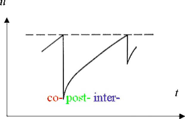
Evolution of displacement during the earthquake deformation cycle.
Évolution temporelle du déplacement lors du cycle sismique.

This concept has guided attempts to predict the date of an earthquake in the future. The time-predictable model states that the time to the next earthquake is the co-seismic slip in the most recent earthquake divided by the fault-slipping rate [107]. An equivalent expression also applies in stress since it is linearly proportional to displacement in an elastic medium such as the Earth's crust. A rigorous statistical application of the linear time predictable model, however, failed to predict the most recent earthquake at Parkfield, California [74]. Nonetheless, the concept of an earthquake deformation cycle provides a contextual framework for interpreting geodetic measurements [111–113].

According to this concept, the vector position x of a benchmark on the ground varies as a function of time t:

x (t) = x (t_{0}) + H (t_{q}) u + (t - t_{0}) v + w (t)

(1)

where

t_{q}

denotes the date (called an ‘epoch’ by geodesists) of an earthquake, u is its co-seismic displacement, H is the Heaviside ‘step’ function that switches from 0 to 1 at time

t_{q}

, v is the inter-seismic velocity, and

w (t)

is a function of time describing the temporal evolution of the post-seismic transient. In the simplest case, if the post-seismic transient is negligible (

w = 0

) and the co-seismic displacement u is the same in each ‘characteristic’ earthquake, then the cycle is periodic (and thus predictable) with a period (or recurrence time)

T = u / v

. The Earth, however, does not always follow such idealized behavior.

To facilitate the discussion, we will make two simplifying assumptions. First, we will assume that the temporal evolution and spatial distribution of the post-seismic transient displacement at time t and vector position coordinate $x_{i}$ is separable (e.g., [36])

W (t, x) = f (t) \times G (x)

(2)

In other words, we can completely describe the spatio-temporal dependence of the post-seismic signal with one map and one time series. This assumption does not apply to models using similarity variables that explicitly couple x and t, such as the stress diffusivity parameter in the Elasser viscous model (e.g., [37]).

Second, we assume that the function $f (t)$ is zero just after the mainshock at time $t_{q}^{+}$ . It then rises to $f (τ) = 1 - 1 / e = 0.63$ after a relaxation time τ and finally to 1 after an infinitely long time interval. Accordingly we can write the total, or fully relaxed, post-seismic displacement field as:

\lim_{t \to \infty} W (t, x) = \lim_{t \to \infty} [f (t)] G (x) = G (x)

(3)

This displacement field records the motion of a point on the ground along its trajectory from the moment $t_{q}^{+}$ just after the earthquake to its final, fully relaxed position.

1.2 Spatial characteristics

When a fault slips seismically, a continuous marker curve, such as a road, becomes discontinuous. Two points that were adjacent at positions $x_{1}$ and $x_{2}$ before the earthquake (at time $t_{1}$ ) are permanently separated in space after the earthquake (at time $t_{2}$ ). The difference in their displacements $u_{1}$ and $u_{2}$ defines the slip vector:

Δ u = u_{2} - u_{1} = [x_{2} (t_{2}) - x_{2} (t_{1})] - [x_{1} (t_{2}) - x_{1} (t_{1})]

(4)

At any single point $x_{i}$ on the ground, a geodetic benchmark, for example, the cumulative displacement over times much longer than the duration of a single earthquake cycle is

u_{i}^{(plate)} = u_{i}^{(inter)} + u_{i}^{(co)} + u_{i}^{(post)}

(5)

as sketched in Fig. 2.

Fig. 2
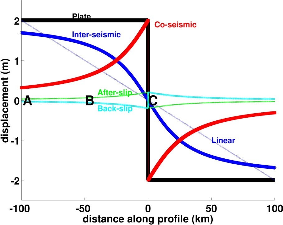
Map view of marker profiles deformed by the earthquake deformation cycle. Once upon a time, the markers, e.g., fence posts, formed a straight line crossing the fault in a right angle. At the time of a single earthquake during the co-seismic interval, the line is offset by the fault rupture (red curve). Then, over the days to centuries of the post-seismic interval, the motion continues in the same sense as co-seismic offset in an ‘after-slip’ mechanism (green curve) or in the opposite sense in a ‘relaxation’ mechanism (cyan curve). The post-seismic curves are discontinuous at the fault if and only if the fault slip reaches the Earth's surface. Over longer times, the deformation returns to its “cruising speed” in the inter-seismic interval (blue curve with arctangent shape). In this case, the fault is locked to a depth of 25 km. Finally, after several million years and many earthquakes, the cumulative displacement recorded in structural geology is a straight line offset at the fault forming the plate boundary (two solid black segments).
Carte d'un profil déformé par le cycle sismique. Autrefois, les marqueurs (par exemple, les poteaux électriques) étaient tous alignés, formant une droite rectiligne qui coupait la faille à angle droit. À l'occasion d'un séisme unique survenant pendant l'intervalle cosismique, la droite est déformée par la rupture de faille (courbe rouge). Puis, pendant l'intervalle post-sismique (quelques jours ou quelques siècles), la déformation continue, soit en afterslip, dans le même sens que l'effet cosismique (trait vert), soit en « relaxation », dans le sens opposé (trait cyan). Les courbes post-sismiques ne sont discontinues à la faille que si la rupture post-sismique atteint la surface de la Terre. Pendant un intervalle de temps encore plus long, la déformation retourne à son « régime de croisière » pendant la phase intersismique (courbe bleu de forme sigmoïdale). Dans ce cas particulier, la profondeur de blocage est de 25 km. Enfin, après plusieurs millions d'années et de nombreux séismes, la géologie structurale enregistre le déplacement cumulé sous la forme de deux droites décalées par rapport à la faille (deux traits noirs).

Over long time intervals, it is convenient to think in terms of rate of displacement, i.e. velocity $v = \partial u / \partial t$ . Accordingly, $v^{(plate)}$ represents the long-term velocity averaged over the last several million years as in the conventional NUVEL-1A plate motion model [26,27]. Note, however, that the above sum applies in displacement u, but not velocity v, because the instantaneous co-seismic displacement $u^{(co)}$ is not differentiable in time. For benchmarks located on the stable, interior parts of continents, where earthquakes are extremely infrequent and fairly small, we may neglect co- and post-seismic displacements. Under these conditions, we expect the long-term velocity $v^{(plate)}$ to approximately equal the inter-seismic velocity $v^{(inter)}$ that we can measure by repeated geodetic surveys. The validity of this approximation has been well confirmed by two global combinations of geodetic velocity estimates including hundreds of benchmarks: ITRF-2000 [3] and REVEL [105]. Except for a few plates (e.g., Nazca and India), differences between the long-term and short-term estimates are within measurement uncertainties. Improved estimates of the terrestrial reference frame are forthcoming and will provide more refined comparisons [28,97].

1.3 Capturing post-seismic transients with satellite geodesy

After having written an expression for the post-seismic deformation field, we now discuss how to measure it using satellite geodesy. Navigation systems such as the Global Positioning System (GPS) estimate the coordinates of a benchmark in some well-defined reference frame. For our purposes, we can consider these three coordinates as an absolute vector position $x (t)$ valid at time t. With multiple surveys, we can determine a time series composed of the three components of the position vector at distinct times. To describe one component of a position time series including an earthquake, we must specify at least three scalar parameters: the initial position $x (t_{0})$ , the inter-seismic velocity v and the co-seismic displacement u. In addition, we would like to estimate at least one more parameter to describe the temporal evolution $f (t)$ part of the post-seismic transient w. For clarity, we will consider several real-world cases.

The first case involves a benchmark that was installed and measured only twice: once before the earthquake, and once again during the excitement following the earthquake. In this case, we have only two data points. Consequently, we can only estimate two parameters, typically $x (t_{0})$ and u. We must assume or neglect the inter-seismic velocity v and the post-seismic transient w. Such a benchmark does not constrain models for post-seismic deformation.

In the second case, we have four data points: two before, and two after, the earthquake. Now we can estimate four parameters: $x (t_{0})$ , u, v, and w. To describe the post-seismic transient w with a single parameter requires assuming a simplest form for $f (t)$ , such as a piece-wise linear ‘triangle’ function of time:

f_{lin} (t) = \frac{(t - t_{q})}{τ_{lin}} when t_{q} < t ⩽ τ_{lin}

(6)

between the time of the earthquake

t_{q}

and some relaxation time

τ_{lin}

. The rest of the time,

f_{lin} (t) = 0

. It reaches 63% of its final, relaxed value when a time interval of

0.63 τ_{lin}

has elapsed after the mainshock.

In the third case, we assume a benchmark that we have been lucky enough to install and survey at least twice before an earthquake occurs. After the earthquake, an increase in funding allows at least three surveys in the post-seismic interval. In this case, we can estimate at least two more parameters to describe a curved shape for the temporal evolution $f (t)$ part of the post-seismic transient w. The shape of the curve depends on the material properties of the Earth's crust, as we will now describe.

2 Rheological analogies

To simplify the discussion, we draw analogies between the continental lithosphere and three mechanical analogs. First, we consider elastic behavior like that of a rubber eraser. Then we consider the effect of pore fluids in analogy with a sponge impregnated with water. Finally, we consider a flowing substrate analogous to honey.

2.1 Rubber eraser analog

In an elastic solid, stress is linearly proportional to strain (Hooke's law). Two coefficients suffice to describe the rheology. Although several different parameterizations appear in the literature, including the bulk modulus k, Young's modulus E, Lamé first coefficient λ, the rigidity μ, and Poisson's ratio ν, any two completely specify the elastic medium. The relationships between these quantities are simple algebraic derivations that appear in many exams and textbooks (e.g., [58]). For simplicity, most studies assume that $λ = μ$ , so that these parameters drop out of the expressions for surface displacement. Such a medium, called a Poisson solid, has a Poisson's ratio ν of 1/4. In this case, the mathematical expressions for displacements, strains and stresses due to fault slip [80] no longer depend on λ, μ, or ν. It is a reasonable approximation because estimates in the upper crust vary from $ν = 0.23$ to $ν = 0.28$ , as inferred from P- and S-wave velocities [30,86]. Poisson's ratio also depends on the amount of fluid included in the rock [117].

The Lamé coefficient μ is called the rigidity in mechanics and the shear modulus in seismology. Typical values (assumed) for rigidity μ in the Earth's crust range from 30 to 36 GPa, but values as low as 10 GPa [25] and as high as 50 GPa [10] have been used. For a fluid, the rigidity is zero because the medium cannot transmit shear stress.

The simplest recipe for describing deformation due to fault slip approximates the Earth as an elastic half space. This formulation has become the conventional standard for modeling co-seismic deformation. Okada [80] derives the expressions for the co-seismic (permanent) displacement at the Earth's surface caused by a slip across a rectangular fault surface at depth in closed analytic form. Accordingly, the surface displacement field $u (x, y)$ due to a dislocation ΔU across a rectangular fault surface with position coordinates ( $x_{f}, y_{f}$ ), width W, length L, strike α, dip δ, buried at depth d in an isotropic elastic medium with Poisson's ratio ν and shear modulus (rigidity) μ below an observing station located at ( $x, y$ ) is:

u (x, y) = Okada (Δ U, ν, μ, L, W, x_{f}, y_{f}, x, y, d, δ, α)

(7)

For the complete set of equations, see Okada's 1985 paper that also corrects previous derivations. In the usual case of a Poisson solid with $ν = \frac{1}{4}$ , the expression no longer depends on ν or μ. For points at depth in the half-space, Okada [81] generalizes the formulation to an arbitrary point located anywhere within in the half-space. Okada's formulation has been applied successfully to over a hundred earthquakes, as reviewed by Feigl [32].

Why is the elastic dislocation formulation so important?

First, it captures the essential physics of deformation due to fault slip in a simple form. During the co-seismic interval, that lasts several hundred seconds at most, the lithosphere behaves elastically. Accordingly, the expressions for displacement u at the surface are linear functions of the fault slip ΔU at depth. This linearity allows us to compute the displacement field for a geometrically complicated fault system as the sum of the displacement fields produced by many smaller, simpler fault elements, or ‘patches’. It also simplifies the inverse problem of estimating the distribution of slip ΔU at depth from geodetic measurements of u at the surface. The half-space approximation appears to be valid for all but the largest earthquakes because the co-seismic displacement exceeds the millimeter level only within a few hundred kilometers of the fault. In other words, the length of the displacement vector $| u |$ falls off steeply with the distance from the station location to the dislocation source. Several recent studies compare the half-space approximation to a radially symmetric spherical Earth model [9,25,75,110].

Second, the parameters in the elastic dislocation model are quantities that we can estimate independently. For example, we can infer the slip ΔU, the length L, and width W of the fault rupture from the seismic moment $M_{0} = μ U L W$ estimated from seismograms [1,43]. This approach involves fewer assumptions than, say, imposing unknown or poorly known forces at far-field boundaries.

Third, the elastic formulation is straightforward to write as computer code. A public-domain computer program written in FORTRAN performs these calculations for an arbitrary observation point on the Earth's surface [33]. Other formulations produce equivalent results [2,40,88,114].

Finally, the elastic dislocation formulation can be extended from the co-seismic case, where it provides an accurate physical description of how faults slip (a ‘model’ in the sense of a prototype or proxy), to other cases, where it can provide an approximate description (a ‘model’ in the sense of a heuristic conceptual analogy). It has become the universally accepted method of choice for calculating co-seismic displacements and slip distributions and has also been widely used to model post- and inter-seismic slip, as we discuss below.

2.2 Eraser analogy for post-seismic deformation

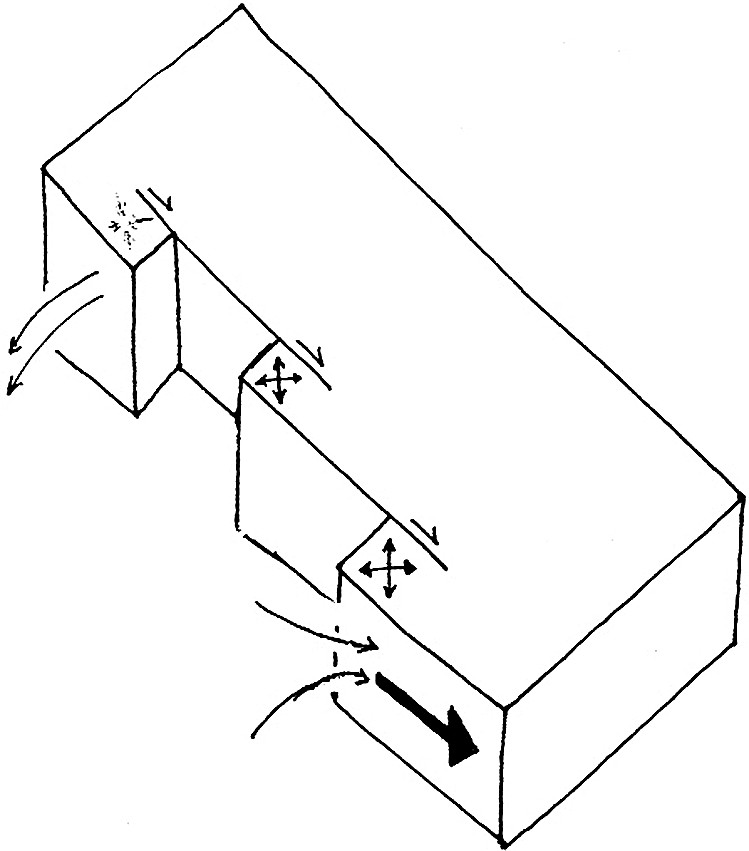
In this mechanism for post-seismic deformation, slip continues in the same plane as the mainshock rupture, as sketched in Fig. 3. An early, well-recorded example appeared in California following the Imperial Valley earthquake of 15 October 1979. In the days following the $M_{w} = 6.5$ mainshock, the fault continued to slip at rates of 5 to 20 mm d⁻¹, diminishing to about 1 mm d⁻¹ ten weeks later [44]. The largest total post-seismic displacements and afterslip rates occurred near the midpoint of the co-seismic surface rupture [44]. Near the northern termination of the co-seismic rupture, the after slip rate averaged $1.08 \pm 0.8 mm d^{−1}$ between 27 October and 13 December 1979 [59]. Two leveling stations, one 5 m west of the fault trace, the other 30 m east, changed their relative vertical elevation by 14 cm (about as much as the co-seismic slip) in the first hundred days after the mainshock [106]. Six weeks after the event, the total post-seismic slip was 8 and 11 cm at two places, representing 13 to 29% of the co-seismic slip, respectively [23]. The overall picture is that afterslip represents continued slip in the same direction as the co-seismic rupture. It seems to be a rapid process with an exponential time scale of 17 days [23], but a logarithmic temporal function also fits the data [59,106]. In many cases, the afterslip is confined to very shallow depths ( $< 1 – 2 km$ ), as the semi-consolidated material near the surface ‘catches up’ to the co-seismic slip at greater depths. The geodetic signature seems to resemble that of creep [24,119].

Fig. 3
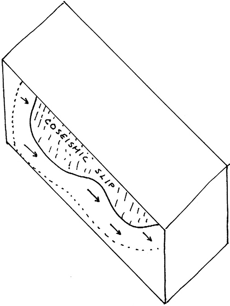
Cartoon of after-slip mechanism analogous to a rubber eraser.
Croquis du mécanisme afterslip analogue à une gomme en caoutchouc.

The 1999 earthquake in Izmit, Turkey provides a complementary example of the post-seismic afterslip, in this case occurring at depths greater than that of the co-seismic slip [15,17,18,31,46,92,120]. Maximum afterslip rates decayed from greater than 5 mm d⁻¹ just after the earthquake to 3 mm d⁻¹ some three months later, with an exponential relaxation time of 57 days [17,31]. In the case of Izmit, the afterslip seems to be considerably deeper than the co-seismic rupture zone. In neither case can the afterslip inferred from the geodetic observations be explained by the recorded aftershocks.

A simple, empirical description of the temporal evolution of post-seismic position is a logarithmic function

f_{\log} (t) = c_{\log} \log [1 + \frac{t - t_{q}}{τ_{\log}}] for t > t_{q}

(8)

where

c_{\log}

is an arbitrary coefficient and

τ_{\log}

is a characteristic relaxation time. At the time of the earthquake

t_{q}

, this function has a value of zero. Afterwards, it rises fairly rapidly, reaching a value of

f_{\log} = 1

when a time interval of

τ_{\log}

has elapsed after the mainshock, providing we have arbitrarily set

c_{\log} = - \log (2)

. One slightly counter-intuitive property of the log function is the trade-off between the two parameters

c_{\log}

and

τ_{\log}

. Only one of them suffices to describe the post-seismic temporal evolution because the logarithmic function can also be written as:

f_{\log} (t) = c_{\log} \log (τ_{\log} + t - t_{q}) - c_{\log} \log (τ_{\log})

(9)

In other words, the final term is already included as the co-seismic offset u in the complete expression (1) for the position coordinate vector $x (t)$ . In practice, we can estimate only one such additive parameter for a given co-seismic epoch in a single coordinate time series.

At longer times, the logarithmic function rises slowly without bound. This is a serious drawback because post-seismic deformation cannot go on forever. One way to handle this shortcoming is to subtract a linear trend from the long-term behavior. The difference between the logarithmic form $f_{\log}$ and the linear form $f_{lin}$ can resemble the exponential form $f_{\exp}$ discussed below. Although the logarithmic functional form seems to fit several post-seismic time series (e.g., station ROCH following Landers [36]), it does not correspond to a simple rheology. It can, however, be related to afterslip in a fault zone with rate- and state-dependent friction [65].

Extending this idea, Perfettini and his colleagues derive a model of brittle creep in the middle layer of the crust above a subduction zone using a rate- and state-friction law [84,85]. Similarly, Kato and others simulate post-seismic deformation on a vertical, strike-slip fault with rate- and state-dependent friction overlying a Maxwell viscoelastic half space [54]. Other studies formulate models along similar lines [60–62]. In its simplest form, a rate- and state-dependent friction law leads to a temporal evolution that shares attributes of the logarithmic and exponential forms. During the early post-seismic interval, it rises quickly, like the exponential form. At later times, however, it continues to rise, like the logarithmic form [36,84].

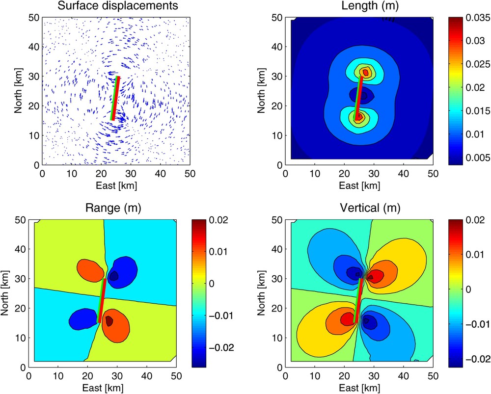
In space, afterslip produces a deformation field with characteristic distance scale on the order of magnitude of the depth at which the post-seismic slip occurred, less than 5 km for Imperial Valley, but 20 to 30 km for Landers and Izmit. Overall, the deformation field produced by post-seismic afterslip resembles the co-seismic field in shape and direction, but with smaller amplitude, with displacement vectors typically $\sim 1 / 10$ as long as their co-seismic values (Fig. 4).

Fig. 4
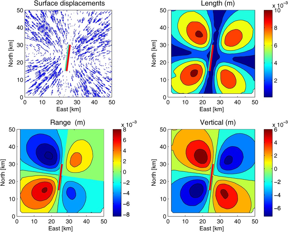
Displacement fields from an after-slip model with 40 cm of right-lateral strike-slip rupture between depths of 10 and 15 km on a fault segment with length 15 km and dip 88°W, showing horizontal displacements (upper left), magnitude of displacement vectors in meters (upper right), INSAR range change in meters for a descending (north–south) pass at latitude 45° (lower left), and the vertical component of displacement in meters (lower right).
Champs de déplacement, d'après un modèle de mécanisme afterslip, supposant 40 cm de glissement en décrochement dextre à une profondeur comprise entre 10 et 15 km sur une faille de 15 km de longueur et de pendage de 88° vers l'ouest. En haut à gauche, les déplacements horizontaux. En haut à droite, la magnitude en mètres. En bas à gauche, le changement de distance qu'enregistrerait un satellite radar en passage « descendant » (du nord vers le sud) à la latitude 45°. En bas à droite, la composante verticale du déplacement, en mètres.

2.3 Sponge analog

Earthquakes change the state of stress in the material around the generative fault, and if the medium is fluid saturated the seismically-induced static stress gradients generate fluid flow that couples into the deformation field. This stress perturbation can be as large as 1–10 MPa (10 to 100 bar) on the fault and decays with increasing distance from each dislocation source. It can affect hydrological conditions, as observed in streams and water wells [71–73]. Hydrothermal activity seems to have changed prior to the 1989 Loma Prieta earthquake in California [108]. The level of water in wells changed during or following the 1999 earthquakes in Turkey [121]. Similar effects were observed in an abandoned mine over several months after a $M_{w} 7.2$ earthquake in Japan [79]. Fountaining of water and sediments was observed during the 2001 earthquake in India [87].

Similarly, several water wells in Iceland began to flow freely (becoming artesian) in the days following the $M_{w} 6.6$ earthquake of 17 June 2000 [12]. Indeed, by mapping the polarity of the change (increase or decrease) in water level over various wells, Icelandic geophysicists were able to recognize the four-quadrant pattern characteristic of a strike-slip earthquake [12,52]. Perturbing the pressure of fluids trapped in the pores, fissures and interstices of rocks alters both their effective elastic moduli and the mechanical behavior of the fault zone itself.

2.4 Poisson recipe for modeling poro-elastic deformation analogous to a sponge

Increasing the fractional fluid volume in a rock changes its rheological behavior. As a result, the ratio $V_{p} / V_{s}$ of seismic wave velocities also changes, in a phenomenon known as dilatancy [39,42,77,101,103,117]. Consequently, the Poisson's ratio and changes with permeability. Assuming that the available pore space in crustal rocks is completely filled with water, Rice and coworkers [21,22,93] derive expressions for Poisson's ratio ν under ‘undrained’ conditions. Such a perturbation in the Poisson's ratio can explain post-seismic deformation over time scales of months and distance scales on the order of 10 km. According to this model, the co-seismic perturbation in the stress field alters the hydrological conditions by changing the fluid pressure instantaneously at time $t_{0}$ , as sketched in Fig. 5. Then, the hydrological conditions readjust as the fluids drain from the interstices and fissures. Eventually, the rock returns to its initial, ‘drained’ condition. The simplest description of this process allows the Poisson's ratio to vary as a function of time. Just after the co-seismic rupture, at time $t_{q}^{+}$ , ‘undrained’ conditions apply:

ν (t_{q}^{+}) = ν_{undrained} = 0.31

(10)

[52,82,83]. At a much later time

t_{1}

, the fluids have drained, decreasing the Poisson's ratio to its usual, ‘drained’ value:

ν (t_{1}) = ν_{drained} = 0.27

(11)

The differential post-seismic displacement accumulated in the interval of time between

t_{q}^{+}

and

t_{1}

is thus:

u_{i} (t_{1}) - u_{i} (t_{q}^{+}) = okada (ν_{drained}) - okada (ν_{undrained})

(12)

since the geometry, the rigidity μ, the slip U are identical in both terms. In other words, this model approximates the post-seismic displacement generated by poro-elastic rebound as the difference between two co-seismic models with different values of Poisson's ratio. Since the undrained Poisson's ratio is generally higher than the drained value, the post-seismic displacement vectors will point in the opposite direction from the co-seismic ones. In map view, Fig. 6 shows that the horizontal displacements produced by the poro-elastic model are similar in magnitude to those produced by the after-slip model. The vertical displacements, however, are opposite in sign. For displacement fields recorded by satellite images, the horizontal and vertical components combine to form an asymmetric range change field. In the Landers case, for example, the projections of the horizontal and vertical components onto the radar line of sight have opposite sign on the east side of the fault, but the same sign on the west side [36].

Fig. 5
Cartoon of Poisson recipe for poro-elastic mechanism analogous to fluid-filled sponge.
Croquis du mécanisme poro-élastique analogue à une éponge engorgée d'eau selon la recette de Poisson.

Fig. 6
Displacement fields calculated using the Poisson recipe. The rupture is 2 m of right-lateral strike-slip between depths of 0 and 15 km on a fault segment with length 15 km and dip 88°. The undrained and drained values of Poisson's ratio are 0.31 and 0.27, respectively. The four panels show horizontal displacements (top left), magnitude of displacement vectors in meters (top right), INSAR range change in meters for a descending (north–south) pass at latitude 45° (bottom left), and the vertical component of displacement in meters (bottom right).
Champs de déplacement calculés selon la formule de Poisson. Le glissement est de 40 cm en décrochement dextre entre 10 et 15 km de profondeur, sur un segment de faille de longueur 15 km et de pendage 88° vers l'ouest. Les valeurs du rapport de Poisson dans les conditions « non-saturé » et « saturé » sont de 0,31 et 0,27, respectivement. En haut à gauche, les déplacements horizontaux. En haut à droite, la magnitude des vecteurs de déplacement, en mètres. En bas à gauche, le changement de distance qu'enregistrerait un satellite radar en passage « descendant » (du nord vers le sud). En bas à droite, la composante verticale du déplacement.

To approximate the displacement field produced by post-seismic deformation of a poroelastic medium, the Poisson recipe takes the difference of two elastic co-seismic models with different values of Poisson's ratio, as described above. This recipe approximates a poro-elastic medium (solid rock and pore fluids) described by four rheological parameters as an elastic medium (analogous to a rubber eraser) described by two elastic parameters. This approximation makes several strong assumptions: (1) that the distribution of co-seismic slip is correct, (2) that the change in Poisson's ratio is spatially uniform, and (3) that the Poisson's ratio changes as a known function of time. At the time of this writing, many modeling studies are focusing on the validity of these assumptions [6,7,14,21,22,36,42,49,52,53,56,67–69,83,93,95,96,102,109,115].

The consequences of this process are challenging to describe, because they depend on local permeability and porosity, which can vary greatly according with rock type, fissure density, porosity and stress. With many simplifying assumptions, one can relate the relaxation time observed in geodetic time series to the hydrologic permeability k. For a fault with width $\sim 1 km$ and a relaxation time of ∼1 month, the permeability should be on the order of $k \sim 10^{−18} m^{2}$ [21]. A more complete treatment, however, requires describing the material parameters with four parameters: two for the solid matrix plus two for the pore fluid [53,116].

The co-seismic perturbation to the hydrologic pressure field also alters the stress conditions on faults near the mainshock, triggering aftershocks where increasing pressure unclamps faults near failure [78]. This mechanism has apparently triggered aftershocks in Iceland [5] and the Afar [76]. By extending the theory to incorporate time-dependent rheology, we should be able to calculate the location of aftershocks triggered by the poro-elastic mechanism of post-seismic relaxation. This approach might also explain changes in the $V_{p} / V_{s}$ ratio observed in the 50 days following the $M w 8.0$ Antofogasta earthquake in Chili in 1995 [56].

2.5 Fault-zone collapse recipe for the sponge analog

Another recipe for describing sponge-like deformation involves a change in volume in the fault zone. For example, Savage et al. [100] proposed a model of ‘fault collapse’ for the 1989 Loma Prieta earthquake. In this case, the source of the post-seismic deformation is modeled as a dislocation with a (negative) tensile component that reduces the volume of a rectangular prism or dike (Fig. 7). One possible physical explanation for this process is the change in widths of cracks and fissures. After opening during the co-seismic rupture, they may slowly heal over the post-seismic interval, with an exponential relaxation time $τ \sim 5 yr$ , as suggested by observations of seismic scattering [8]. The spatial pattern of deformation produced by such a process is shown in Fig. 8. Like the viscoelastic models with a weak substrate (see below), it predicts horizontal displacements perpendicular to the fault plane. Like the Poisson recipe, it predicts short-wavelength features near the fault.

Fig. 7
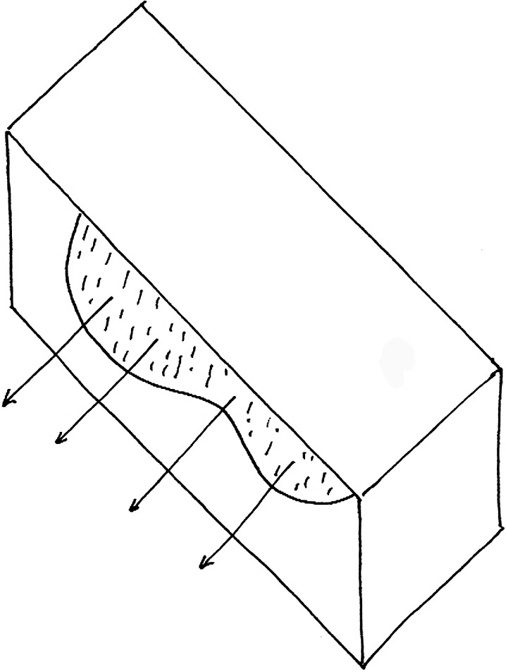
Cartoon of fault-collapse recipe for volume changes in the fault zone analogous to fluid-filled sponge.
Croquis du mécanisme de resserrement de faille, avec changement de volume, analogue au cas d'une éponge engorgée d'eau.

Fig. 8
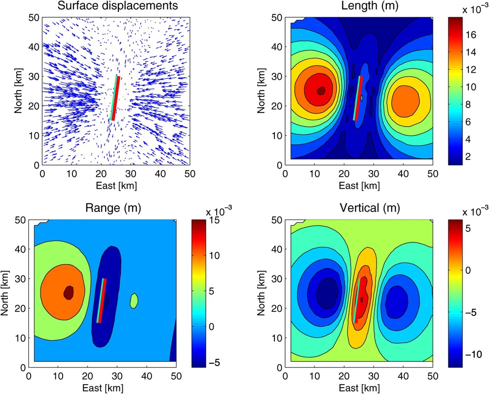
Displacement fields calculated using the fault-collapse recipe. The slip is 40 cm of tensile closing between depths of 10 and 15 km on a fault segment with length 15 km and dip 88°. The four panels show horizontal displacements (top left), magnitude of displacement vectors in meters (top right), INSAR range change in meters for a descending (north–south) pass at latitude 45° (bottom left), and the vertical component of displacement in meters (bottom right).
Champs de déplacement calculés à partir du mécanisme de resserrement de faille. Le glissement est de 40 cm de fermeture ductile sur un segment de faille de 10 à 15 km de profondeur, de longueur 15 km et de pendage 88° vers l'ouest. En haut à gauche, les déplacements horizontaux. En haut à droite, la magnitude en mètres. En bas à gauche, le changement de distance qu'enregistrerait un satellite radar en passage « descendant » (du nord vers le sud). En bas à droite, la composante verticale du déplacement.

Later, Arnadottir et al. [4], concluded that the “geodetic data do not place useful constraints on the amount of dilatancy” for the Loma Prieta event, a conclusion reaffirmed by [16]. However, the fault zone collapse mechanism has not been definitively rejected and has also been proposed for the Landers earthquake [66].

2.6 Honey analog

The third analog considers the lower crust and/or upper mantle as a weak substrate that can flow smoothly. Its rheological behavior is analogous to that of a spoon in honey – movement of the spoon results in flow and permanent, non-recoverable deformation of the honey.

The simplest recipe for describing such flow is a viscous rheology. The stress depends on the strain rate, and if the dependence is linear, the coefficient of proportionality is called the viscosity. Viscosity varies greatly on Earth: $\sim 10^{−5} Pa s$ in air, $\sim 10^{−3} Pa s$ in liquid water, $\sim 10^{9} Pa s$ in glass softened for blowing, and 10¹⁸ to $10^{20} Pa s$ (1 to 100 EPa), in the asthenosphere.

A viscoelastic medium combines viscous and elastic rheologies. There are several possible mechanical combinations that have been applied to study the rheology of Earth's lithosphere. The behavior of a Maxwell solid is analogous to that of a spring and a dashpot connected in series [91]. The spring mimics (recoverable) elastic deformation in the upper crust with an elastic rigidity μ while the dashpot mimics (irrecoverable) viscous flow in the lower crust with a (Newtonian) linear viscosity η. To first order, the displacement signal relaxes exponentially in time over a characteristic ‘Maxwell’ time $τ_{m}$ :

τ_{m} = \frac{η}{μ}

(13)

where some authors include a factor of 2 in the denominator [41]. A rigidity

μ \sim 30 GPa

and a viscosity η of 1 to 100 EPa suggest typical Maxwell times

τ_{m} \sim 1

to 100 years. Other viscoelastic media relevant to post-seismic deformation include the Standard Linear Solid, Burger's body, and tri-viscous media [48].

Estimating the viscosity for rocks at the temperature and pressure conditions prevailing in the Earth is quite challenging. The earthquake deformation cycle is a good rheological experiment because we can measure both the impulse (the co-seismic rupture) and the response (the post-seismic deformation). Other ways of estimating the viscosity in rocks include: laboratory experiments [55], post-glacial rebound [57], gravity studies of lithospheric flexure caused by topographic loading [118] or lacustrine loading [11]. Of course, these estimates of viscosity depend on the assumptions in the models.

2.7 Viscoelastic recipe for honey analog (Fig. 9)

Viscoelastic models for the earthquake cycle generally consist of an upper elastic layer with finite thickness where seismic faulting occurs and one (or more) viscoelastic layer(s) that underlie it. To first order, the viscoelastic model describes the temporal evolution of post-seismic displacement as an exponential function:

f_{\exp} (t) = 1 - \exp (- \frac{t - t_{q}}{τ_{m}})

(14)

where

τ_{m}

is the Maxwell time defined above. Just after an earthquake, at time

t_{q}^{+}

, this function has a value of zero. Then it rises rapidly, it reaches a value of 0.63 after an elapsed time of

τ_{m}

. Assuming effective viscosities ranging from 10¹⁷ to

10^{20} Pa s

, we expect post-seismic displacements driven by viscoelastic processes to decay over a Maxwell time on the order of 1 to 1000 yr. To implement such a viscoelastic rheology for a spherical Earth model, one can sum an infinite series of decaying exponentials (e.g., [89]). If the Maxwell time for the different modes depends on location, however, this formulation will contradict our previous assumption that the time dependence and spatial distribution functions are separable.

Fig. 9
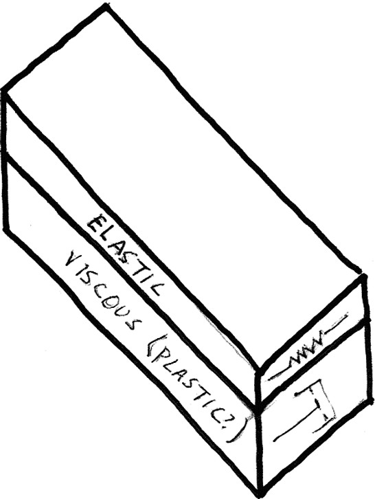
Cartoon of the honey analog, with a brittle-elastic upper crust overlying a weak substrate (lower crust and/or upper mantle) with a viscoelastic or plastic rheology.
Croquis d'un modèle de fluage analogue à celui du miel. La couche supérieure représentant la croûte sismogénique est cassante/élastique. La couche inférieure représentant la croûte inférieure et/ou le manteau supérieur est viscoélastique ou plastique.

The viscoelastic post-seismic displacement field has several distinctive features. For the horizontal components, the co-seismic and post-seismic displacements have the same sign if the viscoelastic source is fairly deep. For the vertical displacements, the co-seismic and post-seismic displacements have opposite signs. This model also tends to produce large displacements perpendicular to the along-strike extension of the fault [102]. The displacement field produced by the viscoelastic relaxation mechanism decays with distance from the fault over length scales on the order of the elastic layer thickness, often taken to be the thickness of part or all of the crust, roughly 10 to 30 km (Fig. 10).

Fig. 10
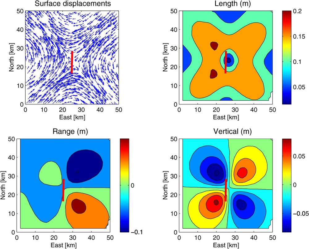
Displacement fields calculated using the viscoelastic recipe for the honey-like mechanism. The initial co-seismic slip is 2 m of right-lateral strike-slip on a fault patch with strike N02°E, dip 87°, length 12 km, and width 6 km. The upper elastic layer has rigidity 30 GPa and Poisson's ratio of 0.27. The lower viscoelastic layer has the same elastic parameters and a viscosity of 3 EPa s. The panels show horizontal displacements (top left), magnitude of displacement vectors in meters (top right), INSAR range change in meters for a descending (north–south) pass at latitude 45° (bottom left), and the vertical component of displacement in meters (bottom right) [29].
Champs de déplacement calculés à partir de la recette viscoélastique pour le mécanisme analogue au cas du miel. Le glissement cosismique initial est de 2 m en décrochement dextre sur un morceau de faille ayant un azimut de N02°E, un pendage de 87°, une longueur de 12 km et une profondeur de 6 km. La couche supérieure est élastique, avec une rigidité de 30 GPa et un rapport de Poisson de 0,27. La couche inférieure viscoélastique se voit attribuer les mêmes valeurs des paramètres élastiques, avec, en plus, une viscosité de 3 EPa s. En haut à gauche, les déplacements horizontaux. En haut à droite, la magnitude, en mètres. En bas à gauche, le changement de distance qu'enregistrerait un satellite radar en passage « descendant » (du nord vers le sud). En bas à droite, la composante verticale du déplacement [29].

Estimating viscosity at depth from geodetic surveys at the surface is difficult because the latter are not very sensitive to the former. Moreover, the trade-offs between depth and viscosity make comparisons between different studies and different areas difficult. Nonetheless, most studies suggest viscosities on the order of 1 to 10 EPa s in the lower crust and/or upper mantle beneath the continents. It seems likely, however, that the weak, flowing substrate obeys a non-linear constitutive relation. For example, aseismic creep on particular sections of some strike-slip faults seems to deform according to a power-law rheology [103,104]. More recently, several studies have suggested power-law rheologies to explain post-seismic deformation [38,90] (Fig. 11).

Fig. 11
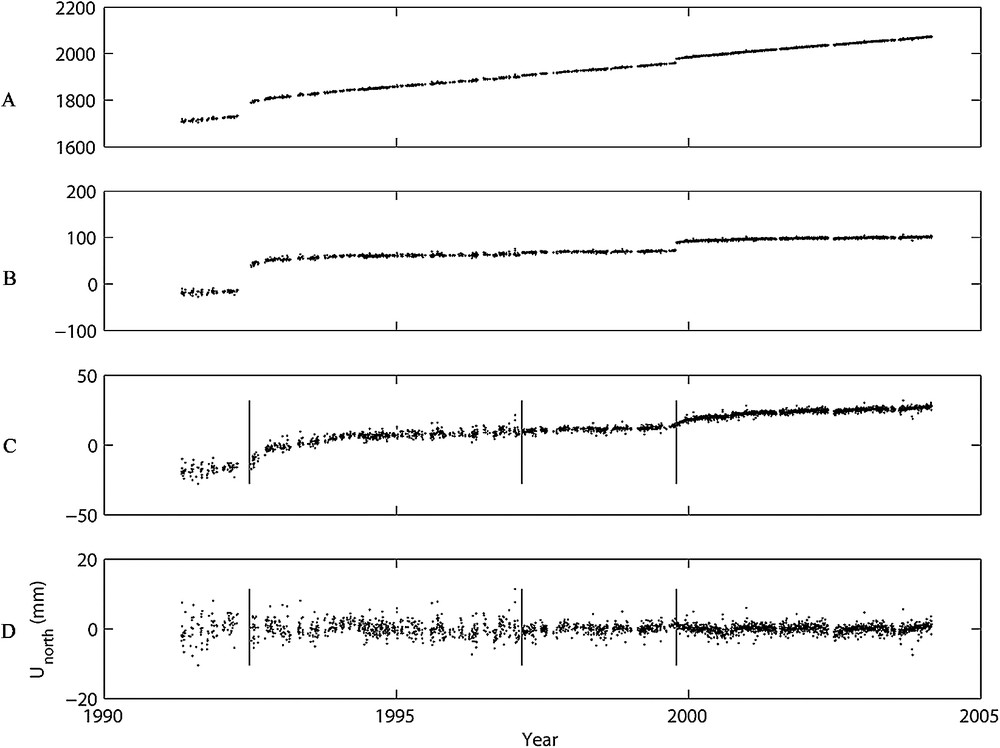
Northing component of position for station ROCH as a function of time. (A) Raw time series realized in a southern California Reference frame from daily solutions by T.A. Herring using SCEC data (personal communication, 2005). Note the three offsets (vertical bars) due to the Landers earthquake in 1992, a change from a Trimble antenna to an Ashtech in 1997, and the Hector Mine earthquake in late 1999. (B) Residuals after removing the best-fitting straight line determined by estimating two parameters. (C) Residuals after removing a straight line and three offsets (five parameters). (D) Residuals after removing a straight line, three offsets, and two logarithmic curves. Error bars not shown for clarity. Outliers more than 10 σ from the piece-wise trend have been omitted.
Composante nord de la position de la station ROCH en fonction de temps. (A) Série temporelle brute réalisée dans un cadre de référence fixe sur la Californie du Sud par T.A. Herring, en utilisant les données SCEC (commun. pers., 2005). Noter les trois décalages (traits verticaux) dus au séisme de Landers en 1992, à un changement d'antenne en 1997 et au séisme de Hector Mine en 1999. (B) Résidus après retrait d'un modèle linéaire avec deux paramètres. (C) Résidus après retrait d'un modèle linéaire avec trois décalages (cinq paramètres libres en tout). (D) Résidus après retrait d'un modèle avec une droite, trois décalages et deux courbes logarithmiques (sept paramètres libres en tout). Les barres d'erreur ne sont pas dessinées. Les points s'écartant du modèle linéaire de plus de 10 écarts-types sont exclus.

3 Tricks of the modeling trade

3.1 Backslip

Savage and Prescott [99] introduced an ingenious shortcut into modeling the surface deformation effects of steady (i.e. constant rate) aseismic fault slip on the downdip extension of the co-seismic fault in elastic and viscoelastic Earth models. They reasoned that the superposition of ‘backwards’ slip (‘backslip’) at constant rate on the shallow co-seismic fault in a sense opposite to co-seismic slip with constant-rate ‘forward’ block motion across the entire fault will produce the same deformation at the Earth's surface as that of a fault locked on its co-seismic segment and freely sliding below. Since the block motion produces no internal strain, the model deformation is due only to the ‘backslip’ element of the model. One calculation then serves to obtain the elastic or viscoelastic effects of any desired distribution of buried steady fault slip, and ‘backslip’ models have become a very popular way of modeling inter-seismic deformation measured by GPS methods, particularly at subducting plate boundaries (e.g., [63]). Johnson and Segall [51] introduced a slightly different formulation using incremental slip that they compare to the standard backslip approach in a helpful sketch (their Fig. 6).

3.2 Distinguishing buried slip from viscoelastic relaxation

Some form of viscoelastic coupling of the largely elastic seismogenic crust and the underlying ductile lower crust or upper mantle must occur and is potentially crucial to understand the earthquake deformation cycle. However, distinguishing the transient buried slip from viscoelastic relaxation from geodetic observations has always been difficult because the observable surface deformation fields produced by the two mechanism are often very similar [111,113]. Indeed, Savage [98] has shown that for a two-dimensional vertical strike-slip fault, the two models are formally equivalent. In this case, an appropriate distribution of elastic dislocations on the fault can superposed to exactly mimic the surface deformation due to relaxation of a viscoelastic half-space lying beneath a faulted elastic plate. For a three-dimensional strike-slip fault this equivalence breaks down: the end effects are of opposite sign for the two models. This diagnostic feature can distinguish the afterslip mechanism from viscoelastic relaxation using INSAR data gathered after the 1999 Hector Mines earthquake [90]. For dip-slip faulting, the two mechanisms are not formally equivalent, even for two-dimensional faults.

4 Synthesis and conclusions

We have considered different mechanisms for explaining post-seismic deformation and arranged them into three categories analogous to a rubber eraser, a sponge, and a spoon in honey. Distinguishing one class of mechanism from another requires considering the temporal evolution and the spatial distribution of the displacement fields they produce. If we assume that the time- and space-dependence of post-seismic deformation are separable, we can describe the observed time series and maps with fairly simple mathematical expressions. The parameters in these expressions vary greatly, however, making it challenging to reject one model in favor of another. Furthermore, more than one process seems to be responsible for producing the post-seismic deformation observed in the seven years following the 1992 Landers earthquake in California. Other earthquakes also suggest different mechanisms acting on different, possibly overlapping, scales in time and space.

Although challenging, the post-seismic problem is well worth pursuing because it represents one of the few rheological experiments that is possible to perform both in situ and in a human lifetime. In the future, we expect progress to come in the following areas:

Robust estimation procedures. We have seen that the parameters in the various models of post-seismic deformation trade off with each other. For example, co-seismic offset will trade off with the characteristic time in a logarithmic function used to describe a time-series of station position. Similarly, estimating viscosity at depth from crustal deformation data measured at the Earth's surface is challenging because the latter is not very sensitive to the former. To obtain robust estimates of these correlated parameters requires estimating them simultaneously in a single optimization procedure. The usual multi-step process of ‘correcting’ the time series for co-seismic offsets and then the inter-seismic rate before curve-fitting the post-seismic part of the time series will bias the estimates of all parameters. Furthermore, if we can assume time–space separability, then we should constrain the temporal evolution function $f (t)$ to be the same at all measurement points. Toward this end, we prefer estimation procedures that “smooth” both the temporal evolution function $f (t)$ and the spatial distribution map $G (x)$ such as GLOBK [47], Network Inversion Filter [104], or Permanent Scatterers [34,35] approaches.

Models that incorporate the geometric complexity of real faults. A normal fault that shallows with depth, as Meyer et al. [69,70] suggest for Grevena, is difficult to approximate with the simple model of a single, planar fault patch. Yet the latter approximation is the most feasible geometric parameterization in the non-linear inverse problem of estimating the focal mechanism [19,20]. Rigo et al. [94] resolved most of this discrepancy by applying a model formulation that admits a non-planar fault surface [64,114]. An open-source computer code for this type of model would foster progress.

More continuous GPS stations. We have seen that time series of geodetic measurements can help to distinguish between various mechanisms for post-seismic deformation. As continuously operating GPS (CGPS) stations become more ubiquitous, they will capture non-linear time series after more earthquakes. The density of CGPS networks in California and Japan (1 station per 1000 km²) should be extended to other fault zones such as the South American cordillera, the boundaries of the Tibetan plateau, and the southwest Pacific. When a large ( $M_{w} > 7$ ) earthquake occurs in an area without dense CGPS coverage, the priority should be installing CGPS instruments in a profile perpendicular to the strike of the co-seismic rupture. For example, if ten instruments are available, five should be installed on each side of the fault with distance of 10 km between them [13,45,50]. If possible, benchmarks near the fault surveyed by campaigns before the earthquake should be equipped with continuously operating instruments. Placing GPS receivers and seismometers in the same locations would save considerable effort.

Routine application of INSAR. To date, several factors make INSAR measurements of transient deformation a hit-or-miss, opportunistic affair. First, the lack of closely spaced orbital trajectories can force a compromise between short time spans (good correlation) and small orbital separation. Second, capturing earthquakes with INSAR is a major challenge because we do not know where they will occur. This implies that each INSAR-capable satellite must acquire a catalog of pre-quake images over all the land areas likely to produce a measurable earthquake. We estimate this area to be approximately 66 million km². A SAR mission dedicated to interferometric measurements of earthquake faulting is needed.

Related phenomena. INSAR and CGPS open two new windows in the spatio-temporal spectrum of seismological metrology: INSAR at distance scales between ∼1 and $\sim 10 km$ ; CGPS at time scales of days to years. Prior to the introduction of these two techniques, measurements at these scales were prohibitively expensive or prone to drift. Now that both techniques have entered the realm of operational, routine observations, we should expect to see interesting observations of other seismological phenomena, such as slow earthquakes, inter-seismic strain accumulation, and perhaps even an earthquake precursor.

Acknowledgements

We thank Jim Savage and Fred Pollitz for critical reviews that significantly improved the manuscript. We also thank Thora Arnadottir, Freysteinn Sigmundsson, Fred Pollitz, Loic Dubois, Dimitri Komatitsch, Hugo Perfettini, Michel Rabinowicz, Brad Hager and Semih Ergintav for helpful discussions. Yuri Fialko, Fred Pollitz, Hugo Perfettini, and Eric Hetland kindly provided results in advance of publication. This work was partially financed by GDR STRAINSAR and ANR.

Bibliographie

[1] K. Abe Moments and magnitudes of earthquakes (J. Ahrens, ed.), Global Earth Physics: A Handbook of Physical Constants, vol. 1, American Geophysical Union, Washington, DC, 1995, pp. 206-213

[2] A. Antonioli; A. Piersanti; G. Spada Stress diffusion following large earthquakes: A comparison between spherical and flat-earth models, Geophys. J. Int., Volume 133 (1998), pp. 85-90

[3] Z. Altamimi; P. Sillard; C. Boucher ITRF2000: A new release of the International Terrestrial Reference Frame for earth science applications, J. Geophys. Res. (Solid Earth), Volume 107 (2002)

[4] T. Arnadottir; P. Segall; M. Mathews Resolving the discrepancy between geodetic and seismic fault models for the 1989 Loma Prieta, California, earthquake, Bull. Seismol. Soc. Am., Volume 82 (1992), pp. 2248-2255

[5] T. Arnadottir; R. Pedersen; S. Jonsson; G. Gudmundsson Coulomb stress changes in the South Iceland Seismic Zone due to two large earthquakes in June 2000, Geophys. Res. Lett., Volume 30 (2003) | DOI

[6] T. Arnadottir; S. Jonsson; F. Pollitz; W. Jiang; K.L. Feigl; E. Sturkell; H. Geirsson Post-seismic deformation following the June 2000 earthquake sequence in the South Icelandic seismic zone, J. Geophys. Res., Volume 110 (2005)

[7] M. Bai On equivalence of dual-porosity poroelastic parameters, J. Geophys. Res., Volume 104 (1999), pp. 10461-410466

[8] S. Baisch; G.H.R. Bokelmann Seismic waveform attributes before and after the Loma Prieta earthquake: Scattering change near the earthquake and temporal recovery, J. Geophys. Res., Volume 106 (2001), pp. 16323-16338

[9] P. Banerjee; F.F. Pollitz; R. Burgmann The size and duration of the Sumatra–Andaman earthquake from far-field static offsets, Science, Volume 308 (2005) no. 5729, pp. 1769-1772 | DOI

[10] S.E. Barrientos; S.N. Ward The 1960 Chile earthquake: inversion for slip distribution from surface deformation, Geophys. J. Int., Volume 103 (1990), pp. 589-598

[11] B.G. Bills; S.L. de Silva; D.R. Currey; R.S. Emenger; K.D. Lillquist; A. Donnellan; B. Worden Hydro-isostatic deflection and tectonic tilting in the central Andes: Initial results of a GPS survey of Lake Minchin shorelines, Geophys. Res. Lett., Volume 21 (1994), pp. 293-296

[12] G. Bjornsson, O.G. Flovenz, K. Semundsson, E.M. Einarsson, Pressure changes in Icelandic geothermal reservoirs associated with two large earthquakes in June 2000, in: Twenty-Sixth Workshop on Geothermal Reservoir Engineering SGP-TR-168, Stanford University, CA, USA, 2001

[13] G. Blewitt Geodetic network optimization for geophysical parameters, Geophys. Res. Lett., Volume 27 (2000), pp. 3615-3618

[14] M. Bonafede Axi-symmetric deformation of a thermo-poro-elastic half-space: inflation of a magma chamber, Geophys. J. Int., Volume 103 (1990), pp. 289-299

[15] A.G. Bos; W. Spakman The resolving power of coseismic surface displacement data for fault slip distribution at depth, Geophys. Res. Lett., Volume 30 (2003)

[16] R. Bürgmann; P. Segall; M. Lisowski; J. Svarc Postseismic strain following the 1989 Loma Prieta earthquake from repeated GPS and leveling measurements, J. Geophys. Res., Volume 102 (1997), pp. 4933-4955

[17] R. Burgmann; S. Ergintav; P. Segall; E.H. Hearn; S. McClusky; R.E. Reilinger; H. Woith; J. Zschau Time-dependent distributed afterslip on and deep below the Izmit earthquake rupture, Bull. Seismol. Soc. Am., Volume 92 (2002), pp. 126-137

[18] Z. Cakir; J.-B.d. Chabalier; R. Armijo; B. Meyer; A. Barka; G. Peltzer Coseismic and early post-seismic slip associated with the 1999 Izmit earthquake (Turkey), from SAR interferometry and tectonic field observations, Geophys. J. Int., Volume 155 (2003), pp. 93-110

[19] P.J. Clarke; D. Paradissis; P. Briole; P.C. England; B.E. Parsons; H. Billiris; G. Veis; J.-C. Ruegg Geodetic investigation of the 13 May 1995 Kozani–Grevena (Greece) earthquake, Geophys. Res. Lett., Volume 24 (1996), pp. 707-710

[20] P.J. Clarke; D. Paradissis; P. Briole; P.C. England; B.E. Parsons; H. Billiris; G. Veis; J.-C. Ruegg Reply to comment by Meyer et al. on “Geodetic investigation of the May 13, 1995 Kozani-Grevena (Greece) earthquake” by P.J. Clarke et al., Geophys. Res. Lett., Volume 25 (1998), pp. 131-134

[21] M. Cocco; J.R. Rice Pore pressure and poroelasticity effects in Coulomb stress analysis of earthquake interactions, J. Geophys. Res., Volume 107 (2002), p. ESE 2-1-ESE 2-17

[22] M. Cocco, J.R. Rice, Corrections to “Pore pressure and poroelasticity effects in Coulomb stress analysis of earthquake interactions”, 2003

[23] C.N. Crook; R.G. Mason; P.R. Wood Geodetic measurements of horizontal deformation on the Imperial Fault (U.S. Geological Survey, ed.), The Imperial Valley, California earthquake of October 15, 1979, Geological Survey Professional Paper, vol. 1254, U.S. Gov. Printing Office, Washington, D.C., 1982, pp. 183-191

[24] T.S. Crough; R.O. Burford Empirical law for fault-creep events, Tectonophysics, Volume 42 (1977), p. T53-T59

[25] G. Dal Moro; M. Zadro Remarkable tilt-strain anomalies preceding two seismic events in Friuli (NE Italy): their interpretation as precursors, Earth Planet. Sci. Lett., Volume 170 (1999), pp. 119-129

[26] C. DeMets; R.G. Gordon; D.F. Argus; S. Stein Current plate motions, Geophys. J. Int., Volume 101 (1990), pp. 425-478

[27] C. DeMets; R.G. Gordon; D.F. Argus; S. Stein Effect of the recent revisions to the geomagnetic reversal time scale on estimates of current plate motions, Geophys. Res. Lett., Volume 21 (1994), pp. 2191-2194

[28] D. Dong; T. Yunck; M. Heflin Origin of the International Terrestrial Reference Frame, J. Geophys. Res. (Solid Earth), Volume 108d (2003)

[29] L. Dubois; K.L. Feigl; D. Komatitsch; T. Árnadóttir Three-dimensional finite-element calculations of co- and post-seismic displacement and stress fields for hazard evaluation in the South Iceland Seismic Zone, EGU, Vienna, 2005

[30] A.M. Dziewonski; D.L. Anderson Preliminary reference Earth model, Phys. Earth Planet. Inter., Volume 25 (1981), pp. 297-356

[31] S. Ergintav; R. Bürgmann; S. McClusky; L. Hearn; R.E. Reilinger; B.A.H. Meteris; B. Aktuk; O. Gurkan; H. Ozener; R. Cakmak; N. Yalcin Postseismic deformation following Izmit Earthquake, 17 August 1999, Bull. Seismol. Soc. Am., Volume 92 (2002), pp. 194-207

[32] K.L. Feigl Measurement of coseismic deformation by satellite geodesy (W.H.K. Lee; H. Kanamoori; P.C. Jennings, eds.), International Handbook of Earthquake and Engineering Seismology, vol. 81A, Academic Press, 2002, pp. 607-620

[33] K.L. Feigl; E. Dupré RNGCHN: A program to calculate displacement components from dislocations in an elastic half-space with applications for modeling geodetic measurements of crustal deformation, Comput. Geosci., Volume 25 (1999), pp. 695-704

[34] A. Ferretti; C. Prati; F. Rocca Nonlinear subsidence rate estimation using permanent scatterers in differential SAR interferometry, IEEE Trans. Geosci. Rem. Sens., Volume 38 (2000), pp. 2202-2212

[35] A. Ferretti; C. Prati; F. Rocca Permanent scatterers in SAR interferometry, IEEE Trans. Geosci. Rem. Sens., Volume 39 (2001), pp. 8-20

[36] Y. Fialko Evidence of fluid-filled upper crust from observations of postseismic deformation due to the 1992 Mw 7.3 Landers earthquake, J. Geophys. Res. (Solid Earth), Volume 109 (2004), p. 08401

[37] G.R. Foulger; C.-H. Jahn; G. Seeber; P. Einarsson; B.R. Julian; K. Heki Post-rifting stress relaxation at the divergent plate boundary in Northeast Iceland, Nature, Volume 358 (1992), pp. 488-490

[38] A.M. Freed; R. Burgmann Evidence of power-law flow in the Mojave desert mantle, Nature, Volume 430 (2004), p. 548

[39] A.M. Freudenthal Shear dilatancy in rock and precursory changes in seismic velocities, Geophys. Res. Lett., Volume 2 (1975), pp. 517-520

[40] J. Gomberg; M. Ellis Topography and tectonics of the central New Madrid seismic zone: Results of numerical experiments using a three-dimensional boundary element program, J. Geophys. Res., Volume 99 (1994), pp. 20299-20310

[41] B.H. Hager; G.A. Lyzenga; A. Donnellan; D. Dong Reconciling rapid strain accumulation with deep seismogenic fault planes in the Ventura basin, California, J. Geophys. Res., Volume 104 (1999), pp. 25207-225219

[42] Y. Hamiel; V. Lyakhovsky; A. Agnon Coupled evolution of damage and porosity in poroelastic media: Theory and applications to deformation of porous rocks, Geophys. J. Int., Volume 156 (2004), pp. 701-713

[43] T.C. Hanks; H. Kanamori A moment magnitude scale, J. Geophys. Res., Volume 84 (1979), pp. 2348-2350

[44] P.W. Harsh Distribution of afterslip on the Imperial Fault (U.S. Geological Survey, ed.), The Imperial Valley, California earthquake of October 15, 1979, Geological Survey Professional Paper, vol. 1254, U.S. Gov. Printing Office, Washington, D.C., 1982, pp. 193-203

[45] E.H. Hearn What can GPS data tell us about the dynamics of post-seismic deformation?, Geophys. J. Int., Volume 155 (2003), pp. 753-777

[46] E.H. Hearn; R. Burgmann; R.E. Reilinger Dynamics of Izmit earthquake postseismic deformation and loading of the Duzce earthquake hypocenter, Bull. Seismol. Soc. Am., Volume 92 (2002), pp. 172-193

[47] T.A. Herring GLOBK: Global Kalman filter VLBI and GPS analysis program version 4.1, Mass. Inst. Technol., Cambridge, MA, USA, 2003

[48] E.A. Hetland; B.H. Hager Postseismic and interseismic displacements near a strike-slip fault: A two-dimensional theory for general linear viscoelastic rheologies, J. Geophys. Res. (Solid Earth), Volume 110 (2005), p. 10401

[49] G. Hillers A strike slip fault model including compaction, dilatancy, and rate and state friction, AGU Fall Meeting Abstracts, Volume 21 (2002), p. 1056

[50] H.O. Johnson; F.K. Wyatt Geodetic network design for fault-mechanics studies, Manuscripta Geodaetica, Volume 19 (1994), pp. 309-323

[51] K.M. Johnson; P. Segall Imaging the ramp-decollement geometry of the Chelungpu fault using coseismic GPS displacements from the 1999 Chi-Chi, Taiwan earthquake, Tectonophysics, Volume 238 (2004), pp. 123-139

[52] S. Jonsson; P. Segall; R. Pedersen; G. Bjornsson Post-earthquake ground movements correlated to pore-pressure transients, Nature, Volume 424 (2003), pp. 179-183

[53] E.F. Kaasschieter; A.J.H. Frijns Squeezing a sponge: A three-dimensional solution in poroelasticity, Comput. Geosci., Volume 7 (2003), pp. 49-59

[54] N. Kato Seismic cycle on a strike-slip fault with rate- and state-dependent strength in an elastic layer overlying a viscoelastic half-space, Earth Planet. Space, Volume 54 (2002), pp. 1077-1083

[55] D.L. Kohlstedt; B. Evans; S.J. Mackwell Strength of the lithosphere: Constraints from laboratory experiments, J. Geophys. Res., Volume 100 (1995), pp. 17587-17602

[56] A. Koerner, S.A. Miller, E. Kissling, A model of deep fluid flow after the 1995 ( $M w = 8.0$ ) Antofagasta, Chile earthquake, EGS–AGU–EUG Joint Assembly, Abstracts from the Meeting held in Nice, France, 6–11 April 2003, abstract #8361, 2003, p. 8361

[57] K. Lambeck; J. Chappell Sea-level change through the last glacial cycle, Science, Volume 292 (2001), pp. 679-686

[58] L.D. Landau; E.M. Lifshitz Theory of Elasticity, Pergamon, Oxford, UK, 1970 (165 p.)

[59] J. Langbein; M.J.S. Johnston; A. McGarr Geodetic observations of post-seismic deformation around the north end of surface rupture (U.S. Geological Survey, ed.), The Imperial Valley, California earthquake of October 15, 1979, Geological Survey Professional Paper, vol. 1254, U.S. Gov. Printing Office, Washington, D.C., 1982, pp. 205-212

[60] N. Lapusta; J.R. Rice; Y. Ben-Zion; G. Zheng Elastodynamic analysis for slow tectonic loading with spontaneous rupture episodes on faults with rate- and state-dependent friction, J. Geophys. Res., Volume 105 (2000), pp. 23765-23790

[61] N. Lapusta; J.R. Rice Nucleation and early seismic propagation of small and large events in a crustal earthquake model, J. Geophys. Res., Volume 108 (2003) no. B4 | DOI

[62] N. Lapusta, J.R. Rice, Earthquake sequences on rate and state faults with strong dynamic weakening, American Geophysical Union, Fall Meeting 2004, abstract #T22A-05

[63] R. McCaffrey; M.D. Long; C. Goldfinger; P. Zwick; J. Nabelek; C. Smith Rotation and plate locking at the southern Cascadia subduction zone, Geophys. Res. Lett., Volume 273 (2000), pp. 3117-3120

[64] F. Maerten, L. Maerten, P. Resor, J. Muller, D. Pollard, A new method for slip inversion for faults with complex geometry, EGS–AGU–EUG Joint Assembly, Abstracts from the Meeting held in Nice, France, 6–11 April 2003, abstract #7473 (2003) 7473

[65] C. Marone; C.H. Scholtz; R. Bilham On the mechanics of earthquake afterslip, J. Geophys. Res., Volume 105 (1991), pp. 8441-8452

[66] D. Massonnet; W. Thatcher; H. Vadon Detection of postseismic fault zone collapse following the Landers earthquake, Nature, Volume 382 (1996), pp. 612-616

[67] T. Masterlark; H. Wang Transient stress-coupling between the 1992 and 1999 Hector Mine, California earthquakes, Bull. Seismol. Soc. Am., Volume 92 (2002), pp. 1470-1486

[68] T. Masterlark; Z. Lu Transient volcano deformation sources imaged with interferometric synthetic aperture radar: Application to Seguam Island, Alaska, J. Geophys. Res., Volume 109 (2004), p. B01401 | DOI

[69] B. Meyer; R. Armijo; D. Massonnet; J.-B. de Chabalier; C. Delacourt; J.-C. Ruegg; J. Achache; P. Briole; D. Panastassiou The 1995 Grevena (Northern Greece) earthquake: fault model constrained with tectonic observations and SAR interferometry, Geophys. Res. Lett., Volume 23 (1996), pp. 2677-2680

[70] B. Meyer; R. Armijo; D. Massonnet; J.-B. de Chabalier; C. Delacourt; J.-C. Ruegg; J. Achache; D. Papanastassiou Comment on “Geodetic investigation on the May 13, 1995 Kozani–Grevena (Greece) earthquake” by Clarke et al., Geophys. Res. Lett., Volume 25 (1998), pp. 129-130

[71] D.R. Montgomery; M. Manga Streamflow and water well responses to earthquakes, Science, Volume 300 (2003), pp. 2047-2049

[72] D.R. Montgomery; H.M. Greenberg; D.T. Smith Streamflow response to the Nisqually earthquake, Earth Planet. Sci. Lett., Volume 209 (2003), pp. 19-28

[73] R. Muir-Wood; G.C.P. King Hydrological signatures of earthquake strain, J. Geophys. Res., Volume 98 (1993), p. 22,035-22,068

[74] J. Murray; P. Segall Testing time-predictable earthquake recurrence by direct measurement of strain accumulation and release, Nature, Volume 419 (2002), pp. 287-291

[75] C. Nostro; A. Piersanti; A. Antonioli; G. Spada Spherical versus flat models of coseismic and postseismic deformations, J. Geophys. Res., Volume 104 (1999), pp. 13115-13134

[76] J. Noir; E. Jacques; S. Bekri; P.M. Adler; P. Tapponnier; G.C.P. King Fluid flow triggered migration of events in the 1989 Dobi earthquake sequence of central Afar, Geophys. Res. Lett., Volume 24 (1997), pp. 2335-2338

[77] A. Nur Dilatancy, pore fluids, and premonitory variations of ts/tp travel times, Bull. Seismol. Soc. Am., Volume 62 (1972), pp. 1217-1222

[78] A. Nur; J.R. Booker Aftershocks caused by pore fluid flow?, Science, Volume 175 (1972), pp. 885-887

[79] H. Ogasawara; Y. Kuwabara; T. Miwa; K. Fujimori; N. Hirano; M. Koizumi Post-seismic effects of an M 7.2 earthquake and microseismicity in an abandoned, flooded, deep mine, Pure Appl. Geophys., Volume 159 (2002), pp. 63-90

[80] Y. Okada Surface deformation to shear and tensile faults in a half-space, Bull. Seismol. Soc. Am., Volume 75 (1985), pp. 1135-1154

[81] Y. Okada Internal deformation due to shear and tensile faults in a half space, Bull. Seismol. Soc. Am., Volume 82 (1992), pp. 1018-1040

[82] G. Peltzer; P. Rosen; F. Rogez; K. Hudnut Postseismic rebound in fault step-overs caused by pore fluid flow, Science, Volume 273 (1996), pp. 1202-1204

[83] G. Peltzer; P. Rosen; F. Rogez; K. Hudnut Poroelastic rebound along the Landers 1992 earthquake surface rupture, J. Geophys. Res., Volume 103 (1998), pp. 30131-30146

[84] H. Perfettini; J.-P. Avouac Postseismic relaxation driven by brittle creep: A possible mechanism to reconcile geodetic measurements and the decay rate of aftershocks, application to the Chi-Chi earthquake, Taiwan, J. Geophys. Res., Volume 109 (2004), p. B02304 | DOI

[85] H. Perfettini; J.-P. Avouac; J.-C. Ruegg Geodetic displacements and aftershocks following the 2001, $M w = 8.4$ Peru earthquake: Implications for the mechanics of the earthquake cycle along subduction zones, J. Geophys. Res., Volume 110 (2005), p. B09404 | DOI

[86] G. Perrier; J.C. Ruegg Structure profonde du Massif central français, Ann. Geophys., Volume 29 (1973), pp. 435-502

[87] B. Pinty; N. Gobron; M.M. Verstraete; F. Mélin; J.-L. Widlowski; Y. Govaerts; D.J. Diner; E. Fielding; D.L. Nelson; R. Madariaga; M.P. Tuttle Observing Earthquake-related dewatering using MISR/Terra satellite data, EOS Trans., Volume 84 (2003), pp. 37-43

[88] D. Pollard; F. Maerten; L. Maerten; P. Resor; J. Muller; A. Aydin Improved 3D modeling of complex fault geometries using Poly3D, an elastic boundary element code, AGU Fall Meeting Abstracts, Volume 21 (2001), p. 0572

[89] F.F. Pollitz Post-seismic relaxation theory on a laterally heterogeneous viscoelastic model, Geophys. J. Int., Volume 155 (2003), pp. 57-78

[90] F.F. Pollitz; C. Wicks; W. Thatcher Mantle flow beneath a continental strike-slip fault: Postseismic deformation after the 1999 Hector Mine earthquake, Science, Volume 293 (2001), pp. 1814-1818

[91] G. Ranalli Rheology of the Earth: Deformation and Flow Processes in Geophysics and Geodynamics, Allen and Unwin, Boston, 1987 (386 p.)

[92] R.E. Reilinger; S. Ergintav; R. Bürgmann; S. McClusky; O. Lenk; A. Barka; O. Gurkan; L. Hearn; K.L. Feigl; R. Cakmak; B. Aktug; H. Ozener; M.N. Toksoz Coseismic and postseismic fault slip for the 17 August 1999, $M = 7.4$ , Izmit, Turkey earthquake, Science, Volume 289 (2000), pp. 1519-1524

[93] J.R. Rice; M.P. Cleary Some basic stress-diffusion solutions for fluid-saturated elastic porous media with compressible constituents, Rev. Geophys. Space Phys., Volume 14 (1976), pp. 227-241

[94] A. Rigo; J.-B. de Chabalier; B. Meyer; R. Armijo The 1995 Kozani-Grevena (northern Greece) earthquake revisited: an improved faulting model from synthetic aperture radar interferometry, Geophys. J. Int., Volume 157 (2004), pp. 727-736

[95] E. Roeloffs Poroelastic techniques in the study of earthquake-related hydrologic phenomena, Advances in Geophysics, Volume 37 (1996), pp. 135-193

[96] P.N. Sahay; T.J.T. Spanos; V. de la Cruz Seismic wave propagation in inhomogeneous and anisotropic porous media, Geophys. J. Int., Volume 145 (2001), pp. 209-222

[97] P. Sarti; P. Sillard; L. Vittuari Surveying co-located space-geodetic instruments for ITRF computation, J. Geodesy, Volume 78 (2004), pp. 210-222

[98] J.C. Savage Equivalent strike-slip earthquake cycles in half-space and lithosphere–asthenosphere Earth models, J. Geophys. Res., Volume 95 (1990), pp. 4873-4879

[99] J.-C. Savage; W. Prescott Asthenosphere readjustment and the earthquake cycle, J. Geophys. Res., Volume 83 (1978), pp. 3369-3376

[100] J.-C. Savage; M. Lisowski; J.-L. Svarc Postseismic deformation following the 1989 ( $M = 7.1$ ) Loma Prieta, California, earthquake, J. Geophys. Res., Volume 99 (1994), pp. 13757-13765

[101] C.H. Scholz; L.R. Sykes; Y.P. Aggarwal Dilatancy, Science, Volume 181 (1973), p. 803

[102] P. Segall; J.-R. Grasso; A. Mossop Poroelastic stressing and induced seismicity near the Lacq gas field, southwestern France, J. Geophys. Res., Volume 99 (1994), pp. 15423-15438

[103] P. Segall; J.R. Rice Dilatancy, compaction, and slip instability of a fluid infiltrated fault, J. Geophys. Res., Volume 100 (1995), pp. 22155-22171

[104] P.A.M.M. Segall Time-dependent inversion of geodetic data, J. Geophys. Res., Volume 102 (1997), pp. 22340-22391

[105] G. Sella; T.H. Dixon; A. Mao REVEL: A model for recent plate velocities from space geodesy, J. Geophys. Res., Volume 107 (2002) (ETG 11-11 to ETG 11-30)

[106] R.E. Sharp; J.J. Lienkaemper Preearthquake and postearthquake near-field levelling across the Imperial fault and the Brawley fault zone (U.S. Geological Survey, ed.), The Imperial Valley, California earthquake of October 15, 1979, Geological Survey Professional Paper, vol. 1254, U.S. Gov't Printing Office, Washington, D.C., 1982, pp. 169-182

[107] K. Shimazaki; T. Nakata Time-predictable recurrence model for large earthquakes, Geophys. Res. Lett., Volume 7 (1980), pp. 279-282

[108] P.G. Silver; J.N. Valette-Silver Detection of hydrothermal precursors to large northern California earthquakes, Science, Volume 257 (1992), pp. 1363-1368

[109] N.H. Sleep; M. Blanpied Creep, compaction and the weak rheology of major faults, Nature, Volume 359 (1992), pp. 687-692

[110] W. Sun Asymptotic solution of static displacements caused by dislocations in a spherically symmetric Earth, J. Geophys. Res., Volume 109 (2004), p. B05402 | DOI

[111] W. Thatcher Nonlinear strain buildup and the earthquake cycle on the San Andreas fault, J. Geophys. Res., Volume 88 (1983), pp. 5893-5902

[112] W. Thatcher The earthquake deformation cycle, recurrence and the time-predictable model, J. Geophys. Res., Volume 89 (1984), pp. 5674-5680

[113] W. Thatcher; J.B. Rundle A viscoelastic coupling model for the cyclic deformation due to periodically repeated earthquakes at subduction zones, J. Geophys. Res., Volume 89 (1984), pp. 7631-7640

[114] A.L. Thomas, A three-dimensional, polygonal element displacement discontinuity computer program with applications to fractures, faults and cavities in the Earth's crust, M.Sci., Stanford, CA, USA, 1993

[115] J.E. Vidale; Y. Li; Y.A. Fialko; E.S. Cochran; G. Peltzer Defining the mechanical fault, AGU Spring Meeting Abstracts, Volume 13 (2004), p. 01

[116] H.F. Wang Theory of Poroelasticity with Applications to Geomechanics and Hydrology, Princeton University Press, Princeton, NJ, USA, 2000

[117] T. Watanabe Effects of water and melt on seismic velocities and their application to characterization of seismic reflectors, Geophys. Res. Lett., Volume 20 (1993), pp. 2933-2936

[118] A.B. Watts, Isostasy and Flexure of the Lithosphere, 2001 (xix $+ 458 p$ .)

[119] R.L. Wesson Dynamics of fault creep, J. Geophys. Res., Volume 93 (1988), pp. 8929-8951

[120] T.J. Wright; E.J. Fielding; B.E. Parsons; P.C. England Triggered slip: observations of the 17 August 1999 Izmit (Turkey) earthquake using radar interferometry, Geophys. Res. Lett., Volume 28 (2001), pp. 1079-1082

[121] G. Yuce; D. Ugurluoglu Earthquake dates and water level changes in wells in the Eskisehir region, Turkey, Hydrol. Earth Syst. Sci., Volume 7 (2003), pp. 777-781

Commentaires - Politique

Ces articles pourraient vous intéresser

Rapid response to the M $_{w}$ 4.9 earthquake of November 11, 2019 in Le Teil, Lower Rhône Valley, France

Cécile Cornou; Jean-Paul Ampuero; Coralie Aubert; ...

C. R. Géos (2021)

Is earthquake activity along the French Atlantic margin favoured by local rheological contrasts?

Yves Mazabraud; Nicole Béthoux; Bertrand Delouis

C. R. Géos (2013)

Volcanic unrest possibilities in response to recent Obruk seismic swarm on and around Hasandağ stratovolcano (Central Anatolia, Turkey)

Erkan Aydar; Caner Diker; İnan Ulusoy; ...

C. R. Géos (2021)