

Version française abrégée
Introduction
Une gestion optimale de l’irrigation, permettrait de réduire la consommation d’eau et le lessivage de nitrates à l’échelle d’une parcelle agricole, mais cela suppose de différencier les apports en fonction des caractéristiques locales des sols. Pour tester des scénarios d’une telle irrigation dite de précision, une méthodologie de simulation fondée sur la modélisation de la variabilité spatiale du sol, des apports et de la culture est nécessaire. La méthodologie testée pour une parcelle agricole consiste (i) à utiliser la géophysique pour accéder à la variabilité spatiale de la profondeur des sols selon un maillage fin, (ii) à effectuer, sur ce même maillage, des simulations stochastiques de l’irrigation et de la réserve utile, (iii) à entrer ces simulations dans un modèle de culture pour en déduire une évaluation spatialisée des transferts d’eau et du rendement. Les mesures de résistivité apparente ont montré leur intérêt pour fournir une description fine, mais indirecte, des variations d’épaisseur et des caractéristiques agronomiques des sols [3,7,11,17,18]. La simulation stochastique spatialisée proposée ici permet de générer conjointement la variabilité spatiale des entrées et des sorties du modèle de culture avec une évaluation de l’incertitude sur les résultats [14,23,28]. Cette méthodologie est testée sur une unité de sols d’une parcelle expérimentale.
Méthode
L’approche stochastique spatialisée utilise des cartes maillées de différentes variables en entrée d’un modèle de culture, obtenues par tirages aléatoires suivant un modèle de loi spatiale statistique ou géostatistique établi à partir de mesures au champ. La modélisation de la profondeur de sol exploite la corrélation spatiale de celle-ci avec la résistivité apparente à travers un modèle linéaire de corégionalisation [8], dans lequel les variogrammes simples et croisés sont des combinaisons linéaires des mêmes composantes élémentaires. Une simulation consiste en un tirage d’un ensemble de variables d’entrée (profondeur de sol, irrigation, et, par couche de sol : teneur en eau initiale, teneur en eau au point de flétrissement et à la capacité au champ) ; cette étape est répétée afin d’obtenir plusieurs réalisations équiprobables des différentes cartes. Appliqué à chacun des tirages, le modèle bidimensionnel STICS [4,5] fournit autant de réalisations équiprobables de cartes des variables de sortie (Fig. 2), décrivant le rendement de la culture et le transfert d’eau et de nitrates. STICS fonctionne au pas de temps journalier et ne prend en compte que les échanges verticaux dans le sol. Les résultats de la simulation sont comparés aux mesures au champ. Une surface d’expérimentation de 1,4 ha (Fig. 1) a été sélectionnée à l’intérieur d’une unité de sol constituée d’horizons argilo-limoneux reposant sur un substrat calcaire [20] à l’intérieur d’une parcelle (X = 592 041 m, Y = 6 768 732 m Lambert 93) de 50 ha, cultivée en maïs grain. Une irrigation optimale de 150 mm a été apportée par pivot, mais une restriction localisée des apports à 60 mm (Fig. 1) permet de tester la méthode pour différentes conditions de stress hydrique.
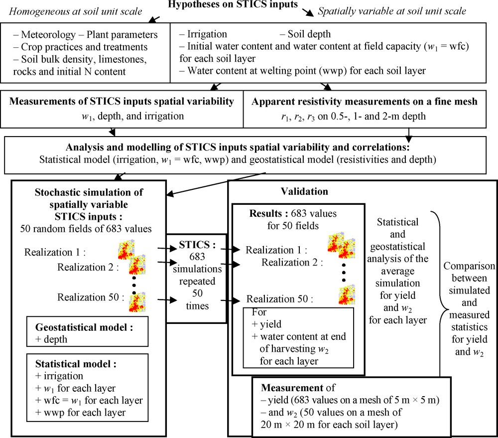
Methodology and model-coupling description.
Fig. 2. Description de la méthodologie et du couplage des modèles.
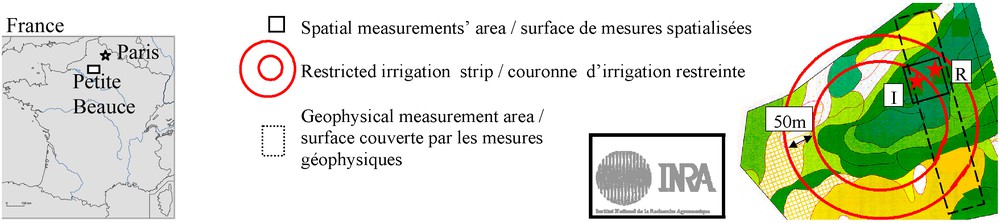
Location of the study (Petite Beauce in France) and description of the network. The pedological map of the studied plot [20] is given, as well as the strip of restricted irrigation water and the sampled areas (R: restricted irrigation; I: abundantly irrigated).
Fig. 1. Localisation de la région d’étude (Petite Beauce en France) et description du protocole. Le fond de carte pédologique de la parcelle d’étude [20] est indiqué, ainsi que l’emplacement de la couronne d’apport d’eau restreint et des surfaces échantillonnées (R : irrigation restreinte ; I : irrigation abondante).
Mesures et simulation des entrées de STICS
La profondeur des sols et les teneurs en eau en début et en fin de culture ont été mesurées aux nœuds d’une grille à maille carrée de 20 m, resserrée localement à 5 m. Les apports d’irrigation ont été mesurés avant la culture tous les 1,25 m le long d’une travée du pivot. La résistivité électrique apparente sur trois profondeurs (0,5, 1,0 et 2,0 m), notée r1, r2 et r3, a été mesurée à maille décimétrique grâce au dispositif MUlti-depth continuous electrical profiling (MUCEP), puis moyennée pour atteindre la maille fine de 5 × 5 m. Le premier facteur de l’analyse en composantes principales de ces trois variables, noté F1r1r2r3, est retenu comme variable auxiliaire de la profondeur de sol. L’irrigation, les teneurs en eau par couche de sol à la capacité au champ en début de culture et celles au point de flétrissement (pF 4,2) sont modélisées par des distributions gaussiennes, centrées sur les moyennes mesurées au champ ou issues des données antérieures [9,10], avec des coefficients de variation égaux aux valeurs expérimentales (Tableaux 1 et 2) ; pour ces variables, la corrélation spatiale n’est pas prise en compte. Les teneurs en eau à la capacité au champ et au point de flétrissement sont supposées corrélées. La profondeur du sol agricole est corrélée au facteur F1r1r2r3 avec un coefficient de détermination de 21 %, la corrélation spatiale croisée étant décrite par le modèle linéaire de corégionalisation (Fig. 3).
Statistics on irrigations (in mm), depths (in m), initial water contents (w1%), and apparent resistivities (r1, r2, and r3, in Ωm)
Tableau 1 Statistiques sur les irrigations (en mm), profondeurs (en m), teneurs en eau initiales (w1 en %) et résistivités apparentes (r1, r2 et r3, en Ωm)
| Statistics | n | m | Min | max | σ | σ 2 | vc | Dist | χ2G (%) | Spatial structure |
| Irrigation | 107 | 11.9 | 9.3 | 14.6 | 1.3 | 1.7 | 0.11 | G | >15 | N |
| Depth | 58 | 0.70 | 0.50 | 1.00 | 0.11 | 0.013 | 0.16 | Gumbel | >15 | Y |
| w1 0–10 | 55 | 21.5 | 14.1 | 25.1 | 2.6 | 6.9 | 0.12 | G | >15 | N |
| w1 10–30 | 55 | 26.4 | 22.9 | 30.7 | 1.8 | 3.2 | 0.07 | G | 5 | N |
| w1 30–50 | 53 | 23.1 | 21.1 | 25.2 | 0.9 | 0.8 | 0.04 | G | 5 | N |
| w1 50–70 | 34 | 23.6 | 22.2 | 25.1 | 0.7 | 0.5 | 0.03 | G | 2,5 | N |
| w1 70–90c | 34 | 18.4 | 12.6 | 23.0 | 2.6 | 6.7 | 0.14 | G | 2,5 | N |
| w1 90–120c | 46 | 17.9 | 14.3 | 21.5 | 2.0 | 4.0 | 0.11 | G | 2,5 | N |
| r 1 | 623 | 24.6 | 21.9 | 27.4 | 1.4 | 1.8 | 0.06 | expG | 15 | Y |
| r 2 | 623 | 35.9 | 30.3 | 40.4 | 2.3 | 5.4 | 0.06 | expG | >15 | Y |
| r 3 | 623 | 46.5 | 40.3 | 51.9 | 2.5 | 6.1 | 0.05 | gumbel | >15 | Y |
Statistics on simulations and measurements for the water contents (w2%) per layer (in cm) at the end of the cultivation and for the corn yield (yi in t/ha) on the zone with water restriction (R) and on the zone abundantly irrigated (I)
Tableau 2 Statistique sur les simulations et les mesures pour les teneurs en eau en fin de culture (w2 en %) par couche (en cm) et pour le rendement en grains (yi en t/ha) sur la zone rationnée (R) et sur la zone irriguée abondamment (I)
| n | min | max | m | σ | n | min | max | m | σ | ||
| Simulations on zone R | Measurements on zone R | ||||||||||
| w2 0–30 | 361 | 15.3 | 20.3 | 17.9 | 0.8 | w2 0–10 | 26 | 14.5 | 19.8 | 16.8 | 1.4 |
| w2 10–30 | 26 | 15.9 | 18.4 | 16.8 | 0.6 | ||||||
| w2 30–50 | 361 | 10.4 | 15.0 | 12.7 | 0.7 | w2 30–50 | 26 | 14.4 | 17.3 | 15.9 | 0.7 |
| w2 50–90 | 361 | 9.8 | 15.5 | 12.8 | 0.9 | w2 50–70 | 7 | 14.7 | 19.3 | 16.7 | 1.4 |
| w2 70–90c | 23 | 11.5 | 18.1 | 15.0 | 1.5 | ||||||
| w2 50–120c | 361 | 4.1 | 13.2 | 8.9 | 1.5 | w2 90–110c | 19 | 13.1 | 20.3 | 15.1 | 1.5 |
| Yi | 361 | 7.7 | 11.6 | 10.0 | 0.6 | Yi | 361 | 7.4 | 12.6 | 9.7 | 0.8 |
| Simulations on zone I | Measurements on zone I | ||||||||||
| w2 0–30 | 312 | 15.4 | 25.2 | 19.8 | 1.6 | w2 0–10 | 24 | 17.6 | 23.6 | 20.1 | 1.5 |
| w2 10–30 | 24 | 17.8 | 21.9 | 20.2 | 1.1 | ||||||
| w2 30–50 | 312 | 11.2 | 18.8 | 14.9 | 1.4 | w2 30–50 | 24 | 17.2 | 21.1 | 19.0 | 1.0 |
| w2 50–90 | 312 | 10.2 | 17.7 | 13.4 | 1.2 | w2 50–70 | 11 | 18.3 | 21.9 | 20.0 | 1.2 |
| w2 70–90c | 18 | 12.5 | 17.9 | 15.1 | 1.6 | ||||||
| w2 50–120c | 312 | 4.3 | 13.8 | 9.0 | 1.6 | w2 90–110c | 18 | 12.3 | 21.2 | 15.6 | 2.4 |
| Yi | 312 | 10.6 | 12.0 | 11.9 | 0.2 | Yi | 312 | 9.0 | 12.0 | 10.8 | 0.6 |
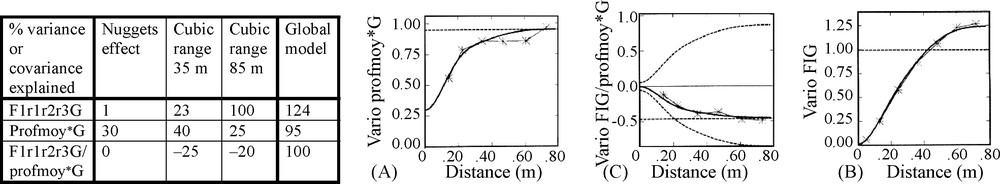
Experimental variogram and variogram model of the Gaussian transform of soil average depth (profmoy*G, graph A in %) and of the Gaussian transform of F1r1r2r3, the PCA first factor for r1, r2, and r3 (F1 G, graph in %). Their cross-variograms are presented on graph C (in %), where are also given curves of the limiting model that verify the constraints on the coregionalization coefficients. The variances and the covariance are normalized by experimental values and are then presented in %. Description of variogram models are indicated with the percent of experimental variance or covariance explained by each model.
Fig. 3. Variogrammes expérimentaux et modèles de variogrammes de la transformée gaussienne de la profondeur moyenne (profmoy*G, graphe A en %) et de la transformée gaussienne du premier facteur d’ACP de r1, r2 et r3 (F1 G, graphe en %). Leurs variogrammes croisés sont présentés sur le graphe C (en %), sur lequel sont aussi indiquées les courbes correspondant aux limites acceptées pour les modèles qui vérifient les contraintes sur les coefficients de corégionalisation. Les variances et la covariance sont normalisées par leur valeur expérimentale et sont donc présentées en %. La description des modèles de variogrammes est indiquée, avec le pourcentage de variance ou de covariance expérimentale expliqué par chaque modèle.
Résultats des simulations
Cinquante simulations ont été effectuées. Les teneurs en eau en fin de culture et le rendement obtenus par simulation ont été comparés aux teneurs en eau mesurées en fin de culture sur le maillage large et au rendement mesuré par l’agriculteur à l’aide d’une moissonneuse équipée d’un capteur de mesure en continu et d’un GPS (Tableaux 1 et 2). Les écarts observés entre les deux situations contrastées d’irrigation ne se retrouvent pas de façon satisfaisante sur les simulations (Tableau 2). Si, pour les teneurs en eau comme pour le rendement, les coefficients de variation (Tableau 2) apparaissent relativement bien conservés, en condition d’irrigation abondante, la variabilité du rendement est lissée, peut-être du fait d’une source de stress ou de variabilité non décrite par le modèle spatialisé. Par ailleurs, les teneurs en eau en fin de culture sont systématiquement sous-estimées dans les couches profondes. La structure spatiale du rendement est correctement restituée. Le coefficient de détermination point par point entre valeurs mesurées et valeurs moyennes des 50 simulations reste faible, mais significatif (37 %).
Discussion et conclusion
Pour la parcelle de Villamblain, les résultats sont encourageants en ce qui concerne l’utilisation des mesures géophysiques pour accéder à la variabilité spatiale structurée de la réserve utile. Cela permettra, dans une seconde étape, de simuler la variabilité spatiale des rendements et des teneurs en eau en fin de culture, en utilisant une modélisation stochastique spatialisée.
Si la variabilité spatiale est assez bien modélisée, les différences entre les valeurs moyennes du rendement et les teneurs en eau du sol simulées en conditions d’irrigation abondante et restreinte sont encore trop imprécises pour permettre une analyse fine de l’effet d’une différenciation à l’échelle de l’unité de sol et pour en tirer des conclusions opérationnelles. Le formalisme du modèle STICS, qui ne prend pas en compte les remontées capillaires, pourrait expliquer en partie ces limitations.
Pour espérer simuler de façon précise une différenciation modérée des irrigations, il est donc nécessaire d’améliorer le modèle de culture en ce qui concerne le bilan hydrique. Il est aussi nécessaire d’affiner les modèles de corrélation entre les variables décrivant l’état du sol, les variables géophysiques et les rendements par des études complémentaires pour différents types de sol, afin de discerner les facteurs de structuration spatiale communs ou prépondérants. Dans l’état actuel, la simulation stochastique spatialisée peut fournir des estimations globales à l’échelle d’une unité de sol, en leur associant une évaluation de l’incertitude associée.
1 Introduction
The development of simulation techniques should make it possible to assess the interest of precision irrigation to optimize the use of water and nitrogen, and to evaluate its possible impact on the crop yield. Precision irrigation consists in varying the water supply as a function of the local characteristics of the soils, as the available water capacity storage (AWSC) inside agricultural plots, and also inside soil units. Indeed irrigation material can adapt the water supply according to a minimum grid of 5 m × 5 m. A methodology based on simulations thus requires description of yield, water, and nitrogen losses as functions of differentiated irrigation carried out according to the soil's water capacity. This modelling requires (i) identification of systematic techniques to assess the spatial variability of the soil water capacity, (ii) description and quantification of the soil spatial variability and of the irrigation variability, and (iii) a suited crop model to obtain differentiated responses.
Among the tools of soil spatial measurements, geophysical methods have already shown their interest for continuous, rapid, and non-intrusive characterisations of soils. Chaplot et al. [7] already demonstrated the advantage of combining several geophysical methods to estimate the spatial distribution of soils affected by water saturation. Nevertheless, a simpler and more rapid method is preferable here. Among the geophysical methods, the apparent resistivity appears as an interesting variable to use as an indicator of the AWSC of agricultural soils [6,7]. Heerman et al. [12] and Dabas et al. [11] also demonstrated the significant part played by the electric variables in the explanation of the crop yield variability. Moreover, the electric method has already shown its sensitivity to soil moisture, and its capacity to distinguish the layers in a pedological context identical to the present one [3,17,18]. The first two metres of the ground in a rural environment usually include an agricultural soil with fine particles and clay overlying a compact bedrock with respectively low and high resistance. The apparent resistitivity of a ground profile thus depends on the resistance as well as on the thickness of the various levels that constitute the profile [3]. Although the apparent resistivity fluctuates partly according to the spatial variability of the agricultural soil resistance, it decreases with the grain size and when the soil porosity, fracturing and/or clay- or water content increase [6,7]. Generally, this corresponds to an increase of the AWSC as if the agricultural soil's depth had increased. Inside a soil unit, where the clay content and coarser materials, such as pebbles, are assumed quite homogeneous, it is supposed that the most important part of the AWSC variability is due to the agricultural soil depth, and is described by the resistivities.
To spatialize a crop model, the simplest method is to carry out a spatial model of entry variables on each mesh of a grid. The method of stochastic simulation [14,23,28] consists in generating random realizations of the same random function, used as input in the crop model. Thus, the corresponding output results make it possible to quantify the uncertainty around their average value [8,16]. In addition, the majority of the soil variables, and in particular, those related to the water transfer, seems to be spatially structured [23,26,29]. The stochastic method is able to take into account the spatial structure by means of geostatistical simulations [8,16]. Lapen et al. [14] used this method to map the risk of crop yield losses according to the spatial variability of soil compaction. It is used here to describe the impact of the spatial variability of the AWSC and irrigation on yield, drainage, and nitrogen leaching.
The present study aims at testing, for an irrigated plot cultivated with maize, (i) the use of geophysical methods to model the main spatial variability of soils depth at a fine scale, and (ii) the coupling of a one-dimensional deterministic agronomic and hydrological model with geostatistical simulations of input variables, in order to carry out a stochastic simulation of the phenomena. First, the methods and tools are presented. The field measurements are used to assess the spatial variability of the variables used as input of the crop model, in order to carry out spatialized stochastic simulations. The simulations results are then compared to field measurements (Fig. 1).
2 Methods and measurement network
2.1 Spatialized stochastic simulation
The method of spatialized stochastic simulation first consists in stochastic simulation of spatially variable inputs of the crop model. Field data are sampled and analyzed by traditional statistical methods [24] and geostatistical tools [16]. Multivariate relations are examined using correlation studies, principal component analysis (PCA) and cross-variograms. Based on this exploratory study, statistical or geostatistical distribution functions are identified for the input variables, taking into account the possible correlations established between them. The simulation consists in a random sampling of a set of variables from their (spatial) distribution, generating a set of input grids with 5 m × 5 m meshes, consistent with potential minimum mesh of differentiation for irrigation. This stage is repeated at least 50 times in order to obtain a significant number of equiprobable realizations of the input mapping (Fig. 2). The software ISATIS [2] was used to build these geostatistical simulations.
To exploit the information brought by the geophysical measurements, a cosimulation is carried out: the soil depth sampled on a broad grid is simulated using the apparent resistivity measured on a fine grid as auxiliary variable. As bivariate model, the linear model of coregionalization is used: all the direct and cross-variograms are a linear combination of the same elementary components. The matrix of the ‘sill’ coefficients of the elementary component must however be positive definite [8].
The method of Gaussian sequential simulation appears convenient here both to take into account geophysical measurements as secondary variables on the fine mesh, and to condition the simulated variable with the measurements on the broader mesh. Conditioning consists in readjusting the simulation with the available experimental variables [8]. It is carried out by adding to the kriging value a random residue with variance equal to the kriging variance. In its simplest version, this method assumes strictly stationary models, that is, of stationary mean value and covariance. In addition, these geostatistical simulations use multiGaussian models [8]. As the variables are generally not Gaussian, it is thus necessary before simulations to transform the variables by anamorphosis, and then to carry out the reverse transformations on the results.
The geostatistical simulations provide 50 realizations for the set of spatially variable input data, on meshes of a grid. For each input realization, the crop model calculates the associated outputs. A significant number (50) of resulting spatialized mappings is then obtained (Fig. 2). This constitutes the stochastic version of the crop model.
2.2 Hypotheses on spatial variability of the STICS model inputs
The agronomic model STICS [4] was chosen to simulate crop yield, drainage, and nitrogen leaching as functions of the following inputs: irrigation, weather, pedological, and agronomic parameters. STICS is a daily time-step reservoir model. It calculates water transfer, neglecting the horizontal exchanges. The hydrodynamic characteristics of the flow are also neglected. Studies of the sensitivity of the model [22,30] showed that the yield and the drainage are particularly sensitive to variations in the irrigation, the initial water content or the AWSC. It was thus assumed that only the spatial variabilities of uncontrolled irrigation, soil depth, initial water content, and water content at the field capacity as well as at the wilting point were to be taken into account in the modelling. The other characteristics of the soil (bulk density of the soil layers, limestone and stone content, initial nitrogen content) were assumed homogeneous at the pedological unit scale.
2.3 Field network
The studied agricultural plot, of an area of 50 ha, is situated in Villamblain (Fig. 1) in the Loiret “département”, in the Petite Beauce (France). Subjected to maritime and continental influences, the regional climate is moderate and rather mild (interannual average of 10.6 °C). The rainfall rate shows a slight deficit: 623 mm for 783 mm of potential evapotranspiration for the years 1967 to 1996. In this area, the slopes are very gentle (2%). The limestone basement contains an aquifer of great thickness whose water table is at a depth of 15 m. A measurement network was set up between March and October 2000 on a crop of maize (Zea mays L., hybrid DK312) irrigated by pivot. The rainfall over the cultivation period from 21st April to 1st October was heavy (311 mm), and the deficit was only 277 mm. Abundant moisture at the period of germination and flowering favored maize growth. On this plot, a study zone of 1.4 ha (Fig. 1) was selected inside a soil unit because of its large surface area and its facies typical of the Petite Beauce region. The soil unit (Calcisol [1]), is made of loamy clay, approximately 70 cm deep, not very stony and calcareous, overlying cryoclastic limestone [20]. The applied amounts of liquid nitrogen were homogeneous throughout the plot (170 kg N/ha). For this first methodological stage, 150-mm irrigation was also carried out homogeneously on the studied area. Nevertheless, in order to test the modelling capacity with different water stress conditions, a restricted irrigation of 60 mm was applied on a circular strip located between 250 and 300 m from the centre of the pivot (Fig. 1). The fitting of the STICS crop model in various conditions of irrigation inputs was carried out in earlier studies [5,9,10,30]. It considered that the roots reach in the limestone a constant depth of 30 cm below the limit of the loamy clay horizon in this type of soils [19].
3 Measurements and simulation of STICS inputs spatial variability
3.1 Measurements
The previously described surface was sampled. Various authors have evaluated the autocorrelation distance of soil parameters related to the water transfer to less than 30 m [15,23,29]. To estimate the variability consistent with this distance, we chose a sampling mesh of 20 m × 20 m, locally decreased to 5 m × 5 m. Soil samples were taken, and analysed by layers of 20 cm, providing description, depth, and gravimetric water content of the soils at the start and at the end of cultivation. The initial water content is assumed to be at the field capacity. Before the harvest, the uncontrolled spatial variability of the irrigation was measured with a step of 1.25 m along the span of the pivot that covers the sampling area.
Measurements of apparent resistivities were taken [26] across an area of 10 ha covering the B zone (Fig. 1) using the device MUCEP [21]. This device is composed of four pairs of toothed wheels used as electrodes. The first pair of wheels serves to inject the current into the ground. The three other pairs, spaced respectively at 0.50, 1, and 2 m, are used as receiving electrodes. The electrodes are connected to a resistivimeter RMCA-4 (EUROCIM-CNRS) located in a vehicle pulling the multipole. The multielectrode device thus allows simultaneous and almost continuous measurements of the apparent resistivity at three increasing depths that correspond roughly to the spacing of the electrodes [26]. These apparent resistivities were noted respectively r1, r2, and r3. The MUCEP was drawn on transects spaced 4.8 m apart, with measurements every 10 cm. After elimination of the aberrant data and filtering by the median method [25], an average value of resistivity was calculated for the 5 m × 5 m mesh.
3.2 Analysis and modelling of irrigation, and water content variability
Irrigation water measurements showed variation coefficients (VC) of about 10% (Table 1) close to those estimated by King et al. [13]. We considered that the observed heterogeneities are preserved in relative values. Although the normality assumption for the irrigation rate was accepted by the Chi2 statistical test [24] with a risk higher than 15%, the uncontrolled variability for each water rotation being described here by a Gaussian distribution centred on the theoretical irrigation of 30 mm, with a standard deviation of 3 mm.
The initial water contents for a 0.20-m thickness was modelled by Gaussian distributions of mean value and standard deviation similar to those measured (Table 1). No correlation between water contents of different layers was taken into account, as none was observed. The water contents at field capacity measured in previous studies [9,10] confirmed that the initially sampled soils reached these water contents. We thus modelled the water contents at field capacity in the same way as the initial water contents. Those at the wilting point are modelled by a Gaussian distribution centred on the previous laboratory measurements [9,10] with the standard deviation measured here at the end of cultivation (Table 2), although those could not be really considered to be at the wilting point.
Partial temporal stability of the water content was assumed because these variables depend on the same physical soil properties. Moreover, Vachaud et al. [27] showed this stability of water contents, measured on a grid and an area similar to those sampled here. The random sampling of water contents at the wilting point was thus partly constrained by relation with the randomly sampled initial water contents, with a covariance supposed equal to the minimum of the measured variances of the initial and final water contents.
3.3 Analysis and modelling of soil depth variability by means of electrical measurements
The depth of the loamy clay layer fluctuates from 0.5 to 1.0 m (Table 1), with a VC of 16%, and was spatially autocorrelated (Fig. 3). The variability of the resistivities was lower with VC ranging between 5 and 7% (Table 1), but highly spatially structured. The PCA between r1, r2, and r3 provided a first common factor, named F1r1r2r3. Depth was significantly correlated with the apparent resistivity at the three measured depths with determination coefficients, equal to the squared correlation coefficient, reaching 21% by using F1r1r2r3. The resistivities were also correlated with the yield with significant determination coefficients of about 16% on the zone, in restricted irrigation conditions. This confirmed that a soil component taken into account in the apparent resistivity partly conditions the crop yield.
The variability of the loamy clay layer thickness was then described with cosimulations using the F1r1r2r3 factor as an auxiliary variable. The fitting of a Gaussian distribution was possible neither for geophysical variables nor for depth measurements (Table 1). We thus carried out Gaussian anamorphoses on the depths and the geophysical variables. The experimental variograms of Gaussian transforms of the thickness and of the F1r1r2r3 factor, and the experimental covariogram of thickness and F1r1r2r3 Gaussian transforms were modelled (Fig. 3) by linear combinations of the same basic models (nugget, cubic of range 35 m, and cubic of range 85 m). The matrix of variance/covariance was verified to be positive definite.
4 Results
4.1 Validation of the method on corn yield and final soil water contents
To evaluate the relevance of the method and of the assumptions adopted for the simulations, a validation of the method was then carried out by comparing the spatialized simulated outputs with field measurements for the cultivation in 2000 (Fig. 2). For example, the estimation of the mean value of a STICS output obtained on the average realization is compared to the mean measured value. We used the corn crop yield measured on a fine mesh, but also the water content at the end of the harvest. To validate the water budget model without drainage data, we indeed compared water contents spatially measured by soil layer at the end of the cultivation to those simulated for the same layers. The crop yield was measured by the farmer by means of a harvester equipped with a differential GPS and sensors of grain volume and moisture, and smoothed on a 5 m × 5 m grid. However, practical simulations can be carried out for periods covering the interculture after harvesting, while those described here only concern the cultivation time span.
The difference between the average yields for each condition of irrigation was overestimated by simulation (Table 2). The statistical variability of the simulated yield described by the standard deviation was completely smoothed in conditions of abundant irrigation (Table 2). On the other hand, in restricted irrigation conditions, the standard deviation and difference between maximum and minimum values for yield were correct, albeit slightly underestimated. Moreover, the simulated yield variogram was quite close to the experimental one and point-to-point correlation between simulated, and measured yield gave a significant determination coefficient of 37%.
The average values of the final soil water content (Table 2) were correctly estimated in the shallow layers, but underestimated at depth, in particular for the deep limestone layers and abundant irrigation. These results were already noticed in the STICS model fitting [30]. The estimated differences between the cases of abundant and restricted irrigation were highly underestimated, particularly in the deep layers. The statistical variability of water contents was fairly evaluated correctly in terms of standard deviation, but differences between maximum and minimum values were overestimated, particularly at depth.
4.2 Discussion
The poor estimates of final soil water contents and differences between yields in varying irrigation conditions showed that the spatial model is not yet able to generate the effects of differentiated irrigation for the studied soils with sufficient accuracy such that the economic impact of precision irrigation can be correctly evaluated in further studies. The results showed that the root water uptake in deep layers is weaker than assumed, and the imprecise responses to water stress and soil variability showed that the STICS model is not sufficiently sensitive to weak variations of water stress and soil characteristics. Indeed, this model was validated with prediction errors of 15% [5] on the variables of interest. The study was however limited to a unit of deep calcosoils, which is probably the most homogeneous zone of the agricultural plot, and for which it is thus difficult to highlight the interest of the precision irrigation at this fine scale.
On the other hand, the validation results showed that the STICS outputs seem adequately described by the spatialized model in spite of STICS model non-linearity, except under abundant irrigation. This confirms the value of stochastic simulations and of geophysical variables used to describe spatial variability of STICS inputs, and their effects on STICS outputs inside a soil unit. This also justifies in part the hypothesis on the choice of major spatially variable STICS inputs and of variability, and correlation models used in the studied case. However, the local estimate was still poor, since the covariance between simulated and measured yield was quite weak. Moreover, in conditions of abundant water, the simulated variability was very low. These points showed that a considerable part of the structured yield variability could not be described by such an elementary use of primary measured electrical resistivities. The complex role of some soil characteristics explains why some spatial structures with a small influence on resistivity can have a major one on the yield, and vice versa. There are probably other sources of variability, such as the amount of rocks, or the water contents in cryoclastic limestones, or the capacity of capillary suction, which has been neglected although they were present. Lastly, the lack of precision of manual soil-depth measurements made by many different observers and the smoothing of yield due to the measurement method itself probably contribute to explain the poor quality of the estimates of yield spatial variability.
5 Conclusion
The spatialization methodology of the STICS crop model developed here included three original and innovative stages, which consisted in testing (i) automated geophysical methods to quickly sample the spatial variability of the AWSC with a fine measurement mesh (5 m × 5 m), (ii) spatialized stochastic simulation methods to evaluate the variability of the estimation made inside a soil unit, (iii) coupling of this stochastic modelling with a crop model, and (iv) automated yield measurements to validate spatially this coupling model on a fine grid.
The methodology proposed here thus appears promising with regard to the geophysical methods to describe the soils at an adequate scale. With regard to the stochastic spatial model, the study shows that spatialization on a minimum scale of irrigation is not yet operative, with a type of water budget model that does not describe capillary rise to simulate the effects of irrigation differentiation at the scale of soils units with high precision. However, the suggested methodology makes it possible to specify uncertainty on the estimation made by neglecting spatial variability inside the soil units.
New assumptions concerning the spatially variable inputs, and their distribution and correlation models to be taken into account will have to be tested to try to improve the estimation in this field and in new case studies. Decomposition of resistivity in a linear combination of soil characteristics must also be tested to determine the influence of each characteristic on the yield spatial variability. Nevertheless, it is also important to improve the capacity of the reservoir model to take into account complex retroactive phenomena, such as capillary suction, before expecting accurate responses to fine differentiation of amounts of irrigation or spatial variability of soils.
Acknowledgements
The authors thank the colleagues who have taken part in the measurements: P. Courtemanche, C. Folton, C. Le Lay, D. Michot, B. Molle, C. Pasquier, S. Renard, B. Renaux, and A.S. Taib. They also thank the two reviewers of an earlier draft of this paper, Dr. C. Gascuel and M. Vauclin, for their help in improving the text.