

1 Introduction
The life cycle of atmospheric pollutants and aerosols depends on emission, transport, chemical transformations, and removal via wet and dry processes [51]. Climate factors enter all these components of the cycle. Emission (e.g., biogenic or dust emissions) may depend on climate variables such as temperature, wind and surface wetness; short and long-term transport depends on the atmospheric circulation and turbulence; chemical transformations depend on temperature, humidity, solar radiation fluxes and cloudiness; wet removal is tied to the precipitation process, and dry removal is essentially driven by turbulent transfer towards the earth's surface. The distribution of pollutants (or more generally chemical tracers and aerosols) is thus strongly dependent on various climatic drivers as well as the distribution of emissions.
Conversely, chemical tracers can affect climate in different ways. For example, greenhouse gases (GHG) absorb infrared terrestrial radiation, while aerosols reflect and absorb solar radiation. Both these processes exert a direct radiative forcing on the climate system, with associated semi-direct effects due to the changes in the atmospheric structure. In addition, aerosols act as cloud condensation nuclei, thereby modifying the microphysical and optical properties of clouds, which in turn can affect climate by the so-called ‘indirect’ effects. It is thus clear that climate–air quality (or more generally climate–chemistry) interactions go in both directions, possibly resulting in feedback mechanisms.
The effects of chemical tracers and aerosols on climate have been extensively investigated by the scientific community for the last few decades [31,32]. However, comparatively less attention has been devoted to the issue of climate-change effects on air quality. In fact, as climate changes, the climatic drivers of the pollutant cycle are also modified and this in turn is expected to affect air quality. As a result, issues of climate change and future air quality are deeply intertwined.
Moreover, climate change–air quality interactions are especially important at the regional scale. Many chemical tracers, in particular those that have negative impacts on human health (e.g., tropospheric ozone and particulate matter) have a relatively short lifetime, in the order of some hours to days [51]. As a result, their distribution is highly variable in space and it is often tied to the distribution of sources. Therefore, a regional context is especially important to investigate climate change–air quality interactions.
Within this context, great improvements have been achieved during the last years in the assessment of regional climate changes due to increased GHG concentrations [32]. This is especially because larger and better quality ensembles of global climate-change projections have become available, from which increasingly robust regional change patterns are emerging [22,24]. In addition, different regionalization techniques have matured to the point of being suitable to provide climate-change information of sufficiently fine scale to capture the spatial detail necessary to investigate air quality issues [25]. As a result, we are now in a better position to assess the effects of climate change on air quality and related regional feedbacks.
Based on these premises, in this paper we present a discussion of modelling the effects of climate change on air quality at the regional scale, where climate change here specifically refers to the effects of anthropogenic forcings (GHG and aerosols) on the climate system during the 21st century. In Section 2, we first summarize the modelling approaches that can be used to investigate regional climate change–air quality interactions. We also present a brief review of previous work in this relatively new specific area of research. This is followed by a discussion of the regional climate-change patterns emerging from the latest generation model simulations (Section 3). In order to illustrate the type of information that can be produced from modelling the effects of climate change on air quality, a specific regional case is presented in Section 4, while final considerations are summarized in Section 5.
2 Modelling the effects of climate change on air quality and brief review of previous work
The simulation of the effects of climate change on air quality requires the use of climate models and air-quality models. In both cases a wide range of models is available that operate both at the global and regional scale [24,25,52,60,61]. Typically, global models have resolutions of the order of a few hundred kilometres and regional models of a few tens of kilometres or less. Climate and air-quality models can be run in the so-called off-line or on-line modes. In the former case, the climate model simulation is run first and the resulting meteorological fields (typically wind, temperature, precipitation, cloudiness, boundary layer height) are used to drive the air-quality model, with no feedback between the tracer concentrations calculated by the air-quality model and the climate fields. In the online approach, the two models are run simultaneously, exchanging information with each other. In the radiatively coupled mode, the meteorological fields drive the air-quality model and the tracer concentrations are fed back to the climate model in order to estimate the related (direct and indirect) radiative effects and climate impacts. In the radiatively uncoupled mode, the meteorological fields drive the air-quality model, but no radiative feedback is allowed for.
Since both climate and air-quality models can be extremely complex modelling systems, the online coupling can be difficult to achieve, both technically and computationally, also because long simulation times are required to assess climate–air quality interactions in a statistically meaningful way. In fact, most online coupled chemistry–climate models used for climate-change simulations include only very simplified representations of chemistry and aerosols, especially when radiative feedbacks are allowed for (e.g., [31,32]). This makes present coupled chemistry–climate models too simple to address air-quality issues, since often changes in air quality depend on very complex interactions between meteorological and chemical factors [51]. As a result, the majority of specific studies of climate-change effects on air quality have adopted the offline approach.
Although a vast literature is available on the general issue of chemistry–climate interactions, only recently some studies have investigated the effects of climate change on air quality. Early studies of climate-change effects on tropospheric chemistry, in particular tropospheric ozone concentrations, include those of Brasseur et al. [4], Johnson et al. [33,34], and of Derwent et al. [10], who used coupled global climate–chemistry models. They found that increased temperature and humidity under global warming conditions would result into a net decrease in total tropospheric ozone concentrations. However, other regional studies [1,53] showed that the warmer temperatures could result in increased near-surface ozone concentrations in urban as well as rural polluted environments.
The first comprehensive studies of the effects of climate change on regional air pollution are those of Hogrefe et al. [29] and Knowlton et al. [37], who focused on regions within the continental United States (USA). They used a regional air-quality model driven off-line by meteorological fields from regional climate model simulations to investigate possible future changes in summer near-surface ozone concentrations over the eastern USA and the New York metropolitan area, respectively. They found an increase in ozone concentration due to climate change alone primarily tied to an increase in biogenic emissions induced by higher temperatures. More importantly, they estimated that this increase is substantial compared to changes in anthropogenic precursor emissions and therefore that climate change is an important aspect to be considered in future air-quality policy planning. Similar results were found in the regional model-based studies of Steiner et al. [55] (for California) and Dawson et al. [8] (for the eastern USA), although the importance of the climate forcing on the ozone concentrations varied in different sub-areas of the regions considered.
Another set of regional model studies available in the literature focus on the European region. Langner et al. [38] and Szopa et al. [58] used regional air-quality models in offline mode to assess the effects of climate change on near-surface ozone concentrations and sulfur and nitrogen deposition over Europe under different GHG emission scenarios. In addition, Forkel and Knocke [14] used an online regional coupled (although not radiatively) atmospheric–chemistry model driven by global model boundary conditions to perform a similar study over southern Germany. All these studies found marked increases of near-surface summer ozone concentrations in response to climate change when assuming no emission control measures. These were attributed to much warmer and drier European summers under future climate conditions. Mixed results were found for the changes in sulfur and nitrogen deposition.
Global model-based studies of climate-change effects on regional air quality are presented by Murazaki and Hess [41], Stevenson et al. [56,57], Shindell et al. [52], Doherty et al. [12]. Murazaki and Hess [41] used a global chemistry model driven by global climate model fields and focused on the effect of climate change on ozone changes in the United States. In a similar fashion to previous regional studies, they found a climate change-induced increase in ozone, particularly over the eastern United States. Stevenson et al. [56,57] and Shindell et al. [52] presented a multi-model study of ozone and carbon monoxide (CO), respectively, using global atmospheric chemistry models run in both offline and online mode. They found a range of responses of ozone and CO to climate change varying across models and future emission scenarios. Finally, Doherty et al. [12] found a significant signature of El Niño on tropospheric ozone and other chemical tracers, again using offline atmospheric chemistry calculations.
All the studies mentioned above clearly indicate that the effects of changes in climatic variables under different global change scenarios are important in determining future pollutant distributions and therefore that climate change needs to be considered as a significant factor in the planning and implementation of future pollution-reduction measures. This factor of course depends on the regional patterns of climate change and can vary from region to region. In the next section, we thus present a discussion of the regional climate-change patterns emerging from the latest generation model simulations.
3 Regional climate-change scenarios emerging from the latest generation model simulations and implications for regional air quality
AOGCMs can provide climate-change information down to subcontinental scales [25]. Recently, 23 AOGCMs from laboratories worldwide were used to complete an unprecedented coordinated set of climate simulations for the 20th and 21st centuries for three IPCC GHG emission scenarios [42] in support of the IPCC fourth assessment report [32 (Chapter 10)]. This dataset is referred to as CMIP3 and it is described and available at http://www-pcmdi.llnl.gov. In this paper, we analyze the CMIP3 dataset for the A1B emission scenario. This scenario lies towards the mid of the full IPCC scenario range, with a CO2 concentration of about 700 ppm by 2100 (near doubling of pre-industrial CO2 concentration). A number of studies (e.g., [17,21,40]) have shown that the spatial patterns of climate change are relatively insensitive to the emission scenario and future time period, with the magnitude of the change signal depending on the magnitude of the GHG concentration and forcing. Therefore, although we only analyze here the A1B scenario, the same conclusions generally apply for other scenarios as well.
Figs. 1–3 show the ensemble mean changes in temperature, precipitation and sea-level pressure (SLP) for December–January–February (DJF) and June–July–August (JJA) in the decades 2071–2100 compared to the reference period 1961–1990. Focusing on the temperature-change patterns first (Fig. 1), we find the well-known signal of more pronounced warming over land areas than oceans. The largest warming occurs at high latitudes and high elevations (e.g., the Himalaya Plateau) in the cold season, because of the melting of snow and sea ice and the effect of the snow-albedo feedback mechanism. Regions where warming appears particularly pronounced are the Mediterranean, central Southwest Asia, the western USA, and the Amazon basin in JJA, the season when temperature is already maximum. Increased temperature implies higher biogenic emissions and faster chemical reactions, both factors being possibly conducive to higher pollutant concentrations.
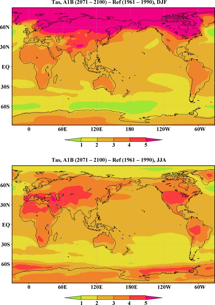
Change in mean surface air temperature for December–January–February (DJF, top panel) and June–July–August (JJA, bottom panel) as simulated by the CMIP3 ensemble. The change is for 2071–2100 compared to 1961–1990, A1B scenario. Units are degrees C.
Fig. 1. Changement de la température moyenne de surface de l’air pour les mois de décembre–janvier–février (DJF, panneau du haut) et juin–juillet–août (JJA, panneau du bas), simulé par l’ensemble CMIP3. Le changement concerne la période 2071–2100, comparée à la période 1961–1990, scénario A1B. Les unités sont exprimées en degrés C.
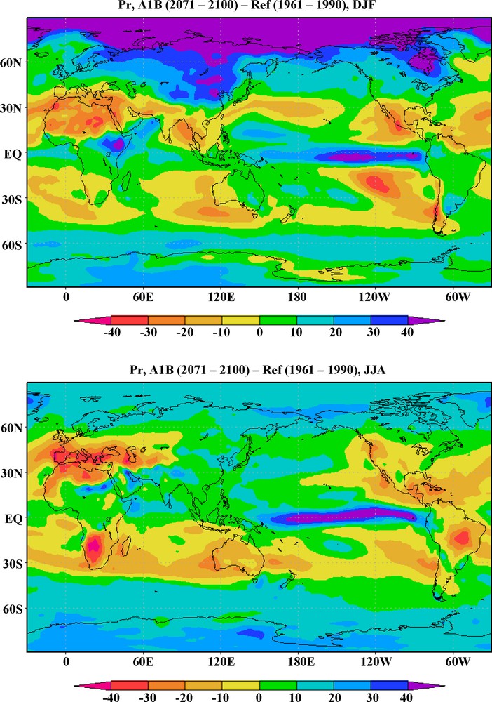
Change in mean precipitation for December–January–February (DJF, top panel) and June–July–August (JJA, bottom panel) as simulated by the CMIP3 ensemble. The change is for 2071–2100 compared to 1961–1990, A1B scenario. Units are % of 1961–1990 values.
Fig. 2. Changement dans les précipitations moyennes pour les mois de décembre–janvier–février (DJF, panneau du haut) et juin–juillet–août (JJA, panneau du bas), simulé par l’ensemble CMIP3. Le changement concerne la période 2071–2100, comparée à la période 1961–1990, scénario A1B. Les unités sont exprimées en pourcentages des valeurs pour les années 1961–1990.
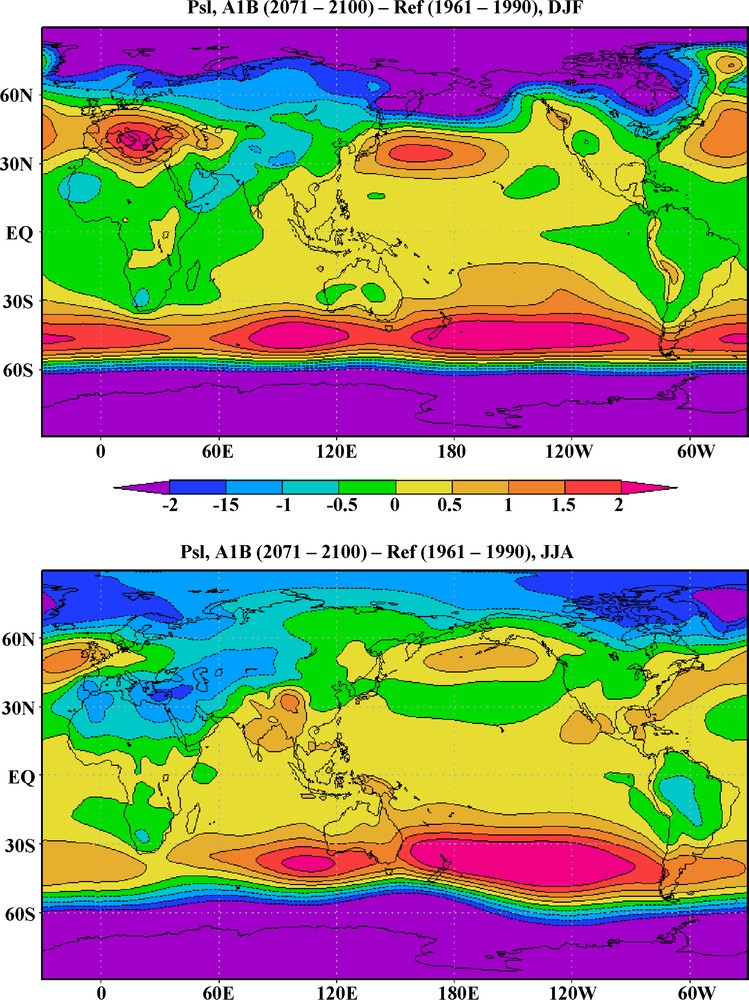
Change in mean sea-level pressure for December–January–February (DJF, top panel) and June–July–August (JJA, bottom panel) as simulated by the CMIP3 ensemble. The change is for 2071–2100 compared to 1961–1990, A1B scenario. Units are hPa.
Fig. 3. Changement dans la pression moyenne du niveau de la mer pour les mois de décembre–janvier–février (DJF, panneau du haut) et juin–juillet–août (JJA, panneau du bas), simulé par l’ensemble CMIP3. Le changement concerne la période 2071–2100, comparée à la période 1961–1990, scénario A1B. Les unités sont exprimées en hectopascals (hPa).
The DJF and JJA precipitation change patterns are shown in Fig. 2. In general, we find increased precipitation at mid to high latitudes and decreased precipitation in the sub-tropics. This is in response to a poleward shift of the mid-latitude storm tracks associated with higher mid-tropospheric warming at the tropics than mid-latitudes, which causes a poleward shift of the Hadley cell and of the areas of maximum meridional temperature gradient [32 (Chapter 10)]. Areas of increased precipitation are also found along the Intertropical Convergence Zone (ITCZ) in response to increased evaporation at the higher temperatures of the climate scenario conditions.
It is useful to highlight some specific regional patterns of precipitation change over land regions. These are most relevant for regional air-quality impacts, because decreased (increased) precipitation would inhibit (enhance) pollutant removal. We find a substantial projected decrease of precipitation over the Mediterranean and Central America, especially in the boreal summer. This should favour pollutant build-up (in particular ozone) because of reduced removal by precipitation and increased photochemistry associated with reduced cloudiness. A substantial decrease of summer precipitation is also found over the western USA (JJA) and the southernmost regions of South America (DJF). By contrast, summer monsoon precipitation is projected to increase over South and East Asia (JJA). Concerning winter precipitation, northern Europe, northern Asia and northern North America show large increases. Conversely, winter precipitation decreases over the Sahara, South and Southeast Asia in the northern hemisphere (DJF), and over southern Africa, Australia and the Amazon basin in the southern hemisphere (JJA).
Fig. 3 shows the changes in SLP, which are an indication of changes in mean circulation. Increases in SLP are indicative of greater subsidence and stagnant conditions, which inhibit pollutant dispersion. Conversely, decreased SLP are generally indicative of increased storm activity and thus increased pollutant dispersion and removal by precipitation. Fig. 3 clearly shows the poleward extension of the Hadley cell and poleward shift of the storm tracks, as evidenced by the decrease in SLP at high latitudes and increase over subtropical regions.
In terms of specific regional SLP change patterns, a prominent one is the pronounced increase in SLP over the Mediterranean region in DJF, which is suggestive of greater subsidence and stagnant conditions over this region. In JJA, we find a blocking high-pressure change pattern off the coasts of northeastern Europe and North America. This causes a northward shift of the storm track impinging upon these continents and the corresponding summer drying observed in Fig. 2. Higher pressure is also found over South Asia and Central America. In the latter case, this results in decreased precipitation (Fig. 2), while in the former it is suggestive of a weakened monsoon circulation, even though monsoon rain increases due to the higher water holding capacity of the warmer atmosphere.
In Section 2 we saw that interannual variability has been found to affect tropospheric ozone concentrations [12]. Previous studies examined projected changes in interannual variability related to increased GHG concentrations [18,19,22,46]. They found a general increase in the variability of precipitation as measured by the coefficient of variation (interannual standard deviation divided by the mean), especially in warm climate regimes. An increase in temperature variability (as measured by the interannual standard deviation) was also found in the warm season and over tropical regions, while a decrease was found in cold climate regimes during the winter season. The increase in variability for warm climate regimes can be attributed to an intensified hydrologic cycle under global warming conditions along with a widespread drying of continental interiors [31,32 (Chapter 10)]. In cold climate conditions, the decrease in variability has been attributed mostly to the decrease of snow cover and the associated snow-albedo feedback process [46].
It is worth noting that an increase in variability along with shifts in the mean (in particular towards warmer conditions) would result in the greater occurrence of extreme seasons (e.g., hot summers). For example, over Europe the incidence of extremely hot summers such as that of 2003 appears much more likely in global warming conditions [48]. This would imply higher frequencies of very high ozone events as seen in the European summer of 2003 [62], which would in turn lead to strong impacts on human health and natural ecosystems (e.g., [45]). In this respect, IPCC [32] concludes that global warming would lead to a widespread increase in the frequency and magnitude of heat waves and drought events, and this would also cause an increase in the occurrence of high pollution events.
To date, RCM-based climate-change simulations have been rather sparse and not very coordinated. Although RCM climate-change scenarios have been run for many regions of the world (e.g., [19,27,64]), these have mostly been isolated efforts that do not allow us to assess the uncertainty related to the scenarios. Only recently, more coordinated RCM climate-change simulation projects have been set up [59]. These projects should eventually provide more robust indications of the fine-scale structure of the climate-change signal, and indeed early simulations do show that complex topography, coastlines and land use locally affect the change in variables such as temperature and precipitation (e.g., [11,16,23,35]). However, many of these coordinated projects are still in their beginning stage, so that an RCM-based comprehensive picture of regional climate change is still not available. The exception to this is the European region, for which the project PRUDENCE [6] has produced a robust assessment of climate change and related uncertainties over this region [9]. In the next section, we thus focus on the European region as an illustrative test bed to study the effects of climate change on air quality.
4 A regional case: climate-change effects on summer air quality in Europe
The European region is one of the most sensitive to climate change [18,19]. Different generations of global and regional model simulations have indicated that the European region is projected to undergo a warming much larger than the global average [9,21,24,36] (see also Fig. 1). Winter precipitation is projected to increase in central to northern Europe and decrease over the southern Mediterranean, while summer precipitation is projected to substantially decrease throughout central-western Europe and the Mediterranean basin [9,21,24,36] (see also Fig. 2). Particularly for the summer climate-change signal, a strong consistency has been found across models, both global and regional [9,24], and these projected European summer climate changes can have important impacts on air quality. In fact, pronounced warming and drying should favour an increase in pollutants such as ozone due to increased biogenic emissions and photochemical rates and reduced wet removal [38,58].
In addition, several studies have suggested that European summer temperature interannual variability might substantially increase in future climate conditions [22,27,48], in particular leading to increased frequency of extremely hot summers (and related high pollution events) such as that of 2003 [22,27,48]. Therefore, summer European climate can be considered as a prominent hotspot in terms of climate change–air quality interactions and an optimal test bed for modelling tools used to investigate them.
Based on these premises, in a separate paper Meleux et al. [39] (hereafter referred to as MSG07) used a state-of-the-art regional CTM to investigate the effects of climate change on summer ozone amounts over the European region. Ozone can be dangerous to human health when very high peak concentrations are reached [44,49] and to ecosystems and agriculture for high chronic exposure [5,15,47]. In this section, we therefore provide a few examples of projected changes in ozone and ozone precursors from the simulations of MSG07 in order to illustrate the potential effect of regional climate change on air quality.
The models used in this study are the regional climate model RegCM [20] and the regional CTM CHIMERE [3,50]. The RegCM modelling system has been used for over a decade in process studies, palaeoclimate and climate-change simulations over different regions of the world [20,28]. The CHIMERE system is routinely used for daily air-quality forecasts over Europe and it is the core of the French air-quality forecasting system Prev’Air. It has also been used for a variety of air-quality studies in different contexts [7]. For the present experiments, a version of CHIMERE is used that does not include aerosol chemistry and microphysics.
It is beyond the purpose of this section to present a detailed analysis of the experiments of MSG07. Rather we only provide some examples of the type of climate change–air quality information that can be achieved with such experiments. By comparison with available observations, MSG07 show that the RegCM-CHIMERE modelling system simulates realistic distribution of near-surface ozone. They also discuss in detail the main factors, both climatic and chemical, affecting the changes in ozone statistics under climate-change conditions. Therefore, the reader is referred to this paper for more information on the experiments and results.
The experimental design of MSG07 follows the offline approach described in Section 2. In order to be run, CHIMERE requires meteorological fields at high temporal resolution (1–6 h). In this case, these are provided by climate simulations with the RegCM described by Giorgi et al. [26,27], which were conducted as part of the PRUDENCE project. RegCM simulated three 30-year periods, 1961–1990 for present-day conditions and 2071–2100 for future conditions under the B2 (low CO2 concentration increase) and A2 (high CO2 concentration increase) GHG emission scenarios of IPCC 2000. The model was driven at the lateral boundaries by corresponding global model simulations (see [26,27] for details). CHIMERE also needs lateral chemical boundary conditions and pollutant emissions. For the former, MSG07 used data from a global CTM climatology (from the MOZART model, [30]), while emissions characteristics for the year 2002 were used for the latter [63]. MSG07 only simulated summer conditions, i.e. out of the full 90 simulated years they extracted summer meteorological data and simulated the corresponding 90 summer seasons (30 for present day, 30 for A2 and 30 for B2) with CHIMERE. Both lateral chemical conditions and anthropogenic emissions are the same in the present day and future air-quality simulations, which allows the isolation of the effects of climate change. Therefore, MSG07 did not take into consideration possible future emission-control policy measures.
Without going into the details of the climate simulations, the experiments of Giorgi et al. [26,27] showed a marked summer warming (up to 3–5 °C) and a reduction of precipitation (up to 30–50%) over the entire European region in the scenario runs compared to present day. This pattern of summer warming and drying was consistent with global [21,24] and regional [9] climate-change simulations and in fact similar to that found in Figs. 1 and 2 for the European region in JJA. It is associated with an intensified anticyclonic ridge over western Europe and the northeastern Atlantic that deflects the summer storm track to the north of western Europe and the Mediterranean [43]. These climate-change conditions are similar to the anomalies found during the summer 2003 over Europe, and this similarity is suggestive of the importance that climate change might have on summer European air quality. Giorgi et al. [26,27] also projected an increase in temperature interannual variability and a decrease in cloudiness. Here we discuss results only for the A2 scenario, for which the CO2 increase is larger (about 850 ppm by 2100) and the change signal stronger [26,27].
Fig. 4 first shows the difference in NOx and isoprene, two critical ozone precursors, between the A2 scenario and present-day simulations in the experiments of MSG07. Both NOx and isoprene increase in the future climate conditions, with this increase showing a marked fine-scale spatial distribution. In the case of NOx (Fig. 4a), we find areas of relatively large increase (2–4 ppb) in correspondence with major metropolitan areas, such as Paris, London, Brussels, and Milan. These are mainly attributed to increased stability (and thus decreased dispersion) associated with an increase in anticyclonic circulation over Europe [43] and to the decrease of the total deposition (wet and dry) of ozone and its precursors.
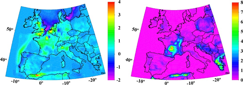
Difference in summer near-surface NOx (a, left panel) and isoprene (b, right panel) daily averaged concentration between the A2 (2071–2100) and present-day (1961–1990) experiments. Units are ppb.
Fig. 4. Différence estivale près de la surface entre les concentrations moyennes journalières de NOx (a, panneau de gauche) et d’isoprène (b, panneau de droite) simulées pour la période A2 (2071–2100) et pour l’époque actuelle (1961–1990). Les unités sont exprimées en parties par milliard (ppb).
Changes in temperature and solar radiation also have a strong effect on biogenic emissions (monoterpenes and isoprene), the only emissions in the simulation which are allowed to vary in response to their dependence on climatic parameters. As Fig. 4b shows, warming and increased solar radiation in the A2 scenario simulation yield a strong increase in isoprene concentrations compared to present day, up to 8 ppb. In addition, in this case we find a marked spatial variability. France exhibits the largest increase in daily averaged isoprene concentration. This biogenic compound plays a key role in ozone production over rural areas, supplying the ozone cycle formation with VOC. Its strong reactivity allows it to produce ozone even in the case of very low NOx concentrations.
Fig. 4 thus shows that ozone precursor availability increases under climate-change conditions. Is this sufficient to affect ozone concentrations? The answer to this question is not obvious, because the warming, circulation changes, increase of humidity and decrease of precipitation and cloud cover will alter the ozone cycle by changing transport, photochemical rates, hydroxyl radical concentration, and PAN distribution.
In the experiments of MSG07, the balance of the effects of all these changes is in the direction of increased ozone concentrations, both for the A2 and B2 scenarios. For example, Fig. 5 shows that the daily averaged ozone concentration increases widely across Europe in the A2 scenario conditions compared to present day. Again, substantial spatial variability in the projected changes is found, with maxima of up to 10 ppb over eastern France and western Germany. Large ozone increases can also be observed over the marine boundary layer in the Atlantic Ocean and over the central Mediterranean around the Marseille area, where summer wind conditions tend to favour ozone accumulation [13].
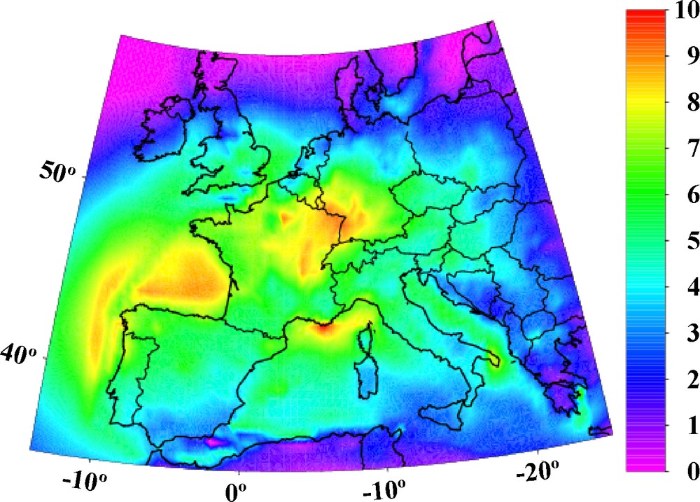
Difference in summer near-surface ozone daily averaged concentration between the A2 (2071–2100) and present-day (1961–1990) simulations. Units are ppb.
Fig. 5. Différence estivale près de la surface entre la concentration moyenne journalière d’ozone simulée pour la période A2 (2071–2100) et pour l’époque actuelle (1961–1990). Les unités sont exprimées en parties par milliard (ppb).
When averaged over the entire European domain, the daily average near-surface ozone amount increases by 7.4% in the A2 scenario compared to present day. Over land, the ozone increase is highly correlated (0.8) with the temperature change and photolysis rate evolutions, but it is also highly correlated (0.9) with the isoprene concentration (see MSG07), thereby identifying isoprene as a key chemical compound responsible for the ozone increase. For the B2 scenario, the increase in ozone has similar patterns, but somewhat smaller magnitude than the A2 one. MSG07 also point out that the ozone levels reached in the A2- and B2-scenario runs are comparable to those found in the summer of 2003, which were much larger than in previous years.
As mentioned, an increase in ozone concentrations should pose an increasing threat to human health, agriculture, and natural ecosystems [15]. Here we illustrate some potential effects of the ozone increase by focusing on the exposure of vegetation and population to ambient ozone. An indicator often used to evaluate vegetation exposure is the AOT40, which is calculated as the sum of the difference between the hourly ozone concentration (ppb) and the 40-ppb threshold, when the concentration exceeds 40 ppb between 8 pm and 8 am [2]. Fig. 6a shows a general increase in AOT40 in our scenario simulations, particularly over France, England, Belgium, the Netherlands, and northern Spain. All these countries are well known for their intensive agriculture, so that an increase in summer ozone concentration due to climate change might pose an increasing threat to agricultural productivity.
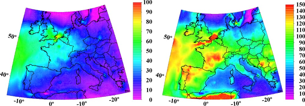
Percentage increase between A2 scenario (2071–2100) and present-day (1961–1990) simulations for the vegetation exposure index AOT40 (a, left panel) and the human exposure index AOT60 (b, right panel). See text for the definition of the indexes.
Fig. 6. Augmentation en pourcentage entre les simulations pour le scénario A2 (2071–2100) et pour l’époque actuelle (1961–1990) des index d’exposition de la végétation AOT40 (a, panneau de gauche) et d’exposition humaine AOT60 (b, panneau de droite). Voir le texte pour la définition des index.
For human health, a corresponding indicator is AOT60 [54], which is calculated in the same way as AOT40, but using a threshold of 60 ppb. For example, when exceeding this threshold, ozone can seriously affect people suffering from respiratory deficiencies [49]. Fig. 6b shows the change in AOT60 calculated for the A2 scenario simulation compared to present day. We see larger increases for AOT60 than for AO40, with similar spatial patterns. AOT60 increases of 80% up to 150% are for example found over France, England, Spain, Portugal, southwestern Germany, Switzerland, Ireland, and Serbia. This indicates that in the experiments of MSG07, very high ozone events show a larger increase than milder events. This may be attributed to the increase in interannual variability mentioned above, which would lead to a much increased occurrence of extreme warm summers.
We should point out two caveats. First, in our simulations, we did not include changes in anthropogenic emissions of ozone precursors, such as NOx. Because of the non-linearity of atmospheric chemistry, such changes might indeed alter the chemical mechanisms leading to ozone formation and thus might (at least partially) change the conclusions found in the present experiments. Second, because of the emphasis on summer ozone, the present version of CHIMERE did not include atmospheric aerosols. However, the chemistry related to aerosol formation and growth could affect the ozone producing mechanisms.
5 Summary considerations and conclusions
The illustrative example shown in the previous section indicates that climate change can have substantial effects on air quality and as a consequence on human health, agriculture, and natural ecosystems. Changes in climatic variables such as temperature, precipitation, circulation, and cloudiness affect the different components of the pollutant life cycle and therefore affect the pollutant concentration. In addition, climate change can be highly variable from region to region, so that the effects of climate change on air quality have to be evaluated from case to case on a regionally specific basis.
This poses an added level of difficulty to the evaluation of climate-change effects on air quality, since projections of regional climate change are still characterized by a relatively high level of uncertainty [32 (Chapter 11)]. However, the emergence of some robust regional climate patterns, the improvement in global and regional modelling tools, and the availability of large multi-model ensembles provide encouraging indications towards increasing our ability to assess climate change–air quality interactions.
Some more specific conclusions can be drawn from present experiments. First, the increase in global and regional temperatures should accelerate the chemical reactions that lead to the formation of pollutants, although this response will likely depend on the non-linearities in the atmospheric chemistry mechanisms. In addition, higher temperatures should increase the biogenic emission of pollutant precursors and this is likely to increase that of atmospheric aerosols. These effects are maximal over regions where the projected warming is maximal, such as continental interiors, high latitudes, and high elevations. Particularly affected by climate change should be the areas projected to undergo a decrease in precipitation, such as the Mediterranean, Central America, the western U.S., southern Africa, and the eastern Amazon basin. This is because increased photolysis rates associated with reduced cloudiness, increased temperatures and reduced wet removal are expected to lead to greater pollutant amounts. Conversely, greater atmospheric cleansing can be expected over areas that are projected to receive increased precipitation amounts, e.g., the high latitude regions. Finally, the projected increase in interannual variability is likely going to lead to higher frequency of extreme climate and pollution events, such as that occurred in the summer of 2003 over Europe.
Our example of section 4 also shows that the effects of climate change on air quality may have a fine-scale detail because of a combination of fine-scale structure in emissions and climatic/chemical factors. Therefore, high spatial resolution is required in order to assess climate change–air quality interactions. In addition, to date climate and air-quality models have been mostly used in offline mode or in online mode, but with no radiative coupling. However, regional feedbacks might be important in determining climate–air quality interactions, especially since major megacities are expected to continue to grow in the future, leading to concentrated high regional emissions. Therefore, the scientific community will inevitably move towards the full on-line radiatively interactive coupling approach, both at the global and regional scales.
A final important consideration is that climate change has an effect on air quality that can be comparable in magnitude, but opposite in sign to that of currently envisioned pollution control measures (see Section 2). Although changes in emission might actually modify the influence of climate change, this still implies that climate change should be an integral part in the design of future emission-control policies. The scientific community is thus faced with the task of providing improved regional climate-change information that can be successfully used in the air-quality policy-decision process.