

1 Introduction
Near-surface ozone, which is a product of the oxidation of anthropogenic and biogenic hydrocarbons and carbon monoxide in the presence of NOx and sunlight, has harmful effects on human health and vegetation. Therefore, numerous efforts have been undertaken to reduce anthropogenic emissions of its precursor compounds in the past. However, changes in regional climate may have an impact on tropospheric ozone concentrations that can possibly negate these mitigation efforts. For central Europe, global climate modelling studies show a trend towards higher temperatures and several models indicate a decrease of cloudiness and precipitation in summer (e.g., [19]). These meteorological conditions can result in an enhanced ozone tropospheric formation.
A number of modelling studies were performed to investigate the development of tropospheric ozone under changed climate conditions on the global scale (e.g., [3,16,23,24,29,31,34,37]. As far as unchanged anthropogenic emissions were considered, these studies indicate increased ozone concentrations under changed climate conditions for polluted regions such as North America, East Asia, or Europe.
Besides the meteorological conditions, the regional distribution of ozone depends strongly on the spatial distribution of precursor emissions. Due to the nonlinear behaviour of atmospheric chemistry, the tropospheric ozone production is different, depending on whether the separation of polluted urban and rural regions is resolved or not [39]. Therefore, the coarse horizontal resolution of current global climate–chemistry simulations does not permit a detailed estimate of the effects of climate change on tropospheric photooxidant distributions on the regional scale. Failure to account properly for inhomogeneities in concentrations of precursor gases and their oxidants can lead to errors in estimates of ozone concentrations and their sensitivities to control strategies [10]. By comparing global model simulations with different horizontal resolutions between T21 (5.6° × 5.6°) and T106 (1.1° × 1.1°), Wild and Prather [45] found that the simulated ozone production close to continental emission regions was significantly overestimated for coarse resolutions and that convergence was not yet achieved for T106.
So far, only few investigations were published on the potential effect of future global climate change on the distribution of photooxidants on the regional scale [5]. Regional simulations for present-day and future climate conditions with 36-km grid spacing by Hogrefe et al. [18] have shown that climate change has a significant impact on the occurrence of high ozone concentrations in the eastern United States. Langner et al. [28] performed regional simulations with a horizontal resolution of 0.8° for two climate scenarios to study the impact of climate change on surface ozone over Europe.
Numerous studies focus on the impact of grid resolution on the results of regional air quality simulations for episodes (e.g., [2,10,20,22,30]). An upper limit of 20–30-km grid resolution was already recommended by Gillani and Pleim [10] for air-quality simulations for the eastern USA. Cohan et al. [2] found that, though first order sensitivities to NOx emissions were largely consistent for 36-, 12-, and 4-km resolution, only a resolution of 12 km or better could capture the extent of VOC sensitivity in the considered region. However, for climate simulations, it is difficult to satisfy the requirements formulated in these studies, as simulation times of 10 years or more are necessary in order to obtain reliable results. So far, the impact of model resolution on the simulated changes of near-surface pollutant concentrations was not an issue in regional climate chemistry investigations.
To investigate the potential impact of changed climate conditions on the regional photosmog situation over central Europe and the results’ sensitivity to model resolution, climate–chemistry simulations with two different resolutions were made with the coupled 3-dimensional meteorology–chemistry model MCCM [6,12]. The simulations for the present-day and a possible future climate scenario were carried out for two nested domains with horizontal resolutions of 60 and 20 km, respectively. These results permit a first estimate of the effect of different grid resolutions on the simulated impact of a climate change scenario on tropospheric ozone on the regional scale.
2 Methods
2.1 General setup
The approach applied in this study is based on dynamical downscaling of a global climate scenario with a regional model. The regional simulations with the climate–chemistry MCCM [6,12] were forced by meteorological boundary conditions that were derived from the output of a 240-year run of the global climate model ECHAM4 [36] coupled with the ocean circulation model OPYC [33]. In two consecutive one-way nesting steps, the global simulation with resolution T42 (about 250–300 km) was downscaled to a resolution of 60 km for Europe and 20 km for central Europe. Fig. 1 shows the domains for the regional simulations.
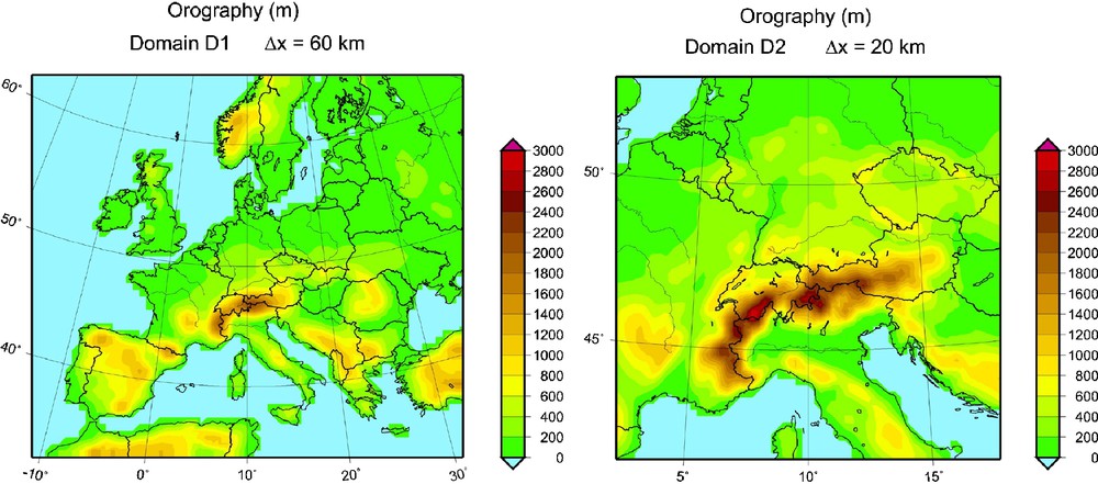
Model domains D1 (60-km resolution) and D2 (20-km resolution), including the representation of the topography.
Fig. 1. Domaines D1 (résolution de 60 km) et D2 (20 km de résolution) du modèle, incluant la représentation de la topographie.
The first domain with a horizontal resolution of 60 km (D1, 66 × 59 grid points) receives meteorological boundary conditions derived from the ECHAM4 output, while chemistry boundary conditions are prescribed. The second domain, with a 20-km resolution (D2, 64 × 64 grid points), receives meteorological and chemistry boundary conditions from the output of the 60-km simulation. In the vertical, the atmosphere between the surface and the 100-hPa level is resolved in 25 layers, the lowest being about 14 m thick. The lower boundary of the 5-layer soil model is located at a depth of 3 m.
As it was the purpose of these simulations to investigate the impact of changes in the meteorological conditions on near-surface ozone, no trends were assumed in anthropogenic emissions and in the prescribed chemistry boundary conditions at the outer boundary of domain D1.
Two time slices were considered, which represent the 90ths of the previous century (‘present’) and the 30ths of this century (‘future’). The simulations start in November of the years 1990 and 2030, respectively. The first two months serve as spin-up time for the meteorological variables and for soil temperature and moisture as well as snow depth. The simulations were carried out continuously until December 2000 and December 2039, yielding 10 and 9 years of model output for the subsequent analysis.
2.2 The regional climate chemistry model MCCM
The online coupled regional meteorology–chemistry model Mesoscale climate chemistry model (MCCM) [6,12] is based on the non-hydrostatic NCAR/Penn State University mesoscale model MM5 [11]. MCCM predicts the relevant meteorological processes, soil temperature and moisture, as well as chemical transformations in the gas phase and optionally particle phase processes. Like MM5, MCCM supports multiple nesting of domains and can be applied over a spatial scale ranging from the continental scale with domain extensions of several thousands of kilometres and resolution of 30–100 km down to the regional scale, with domains of 100–200 km and resolutions of 1–5 km. MCCM includes a choice of different online coupled tropospheric gas phase chemistry modules (RADM [41], RACM [42], and RACM-MIM [9]). Optional aerosol processes are described by a modal approach with the MADE/SORGAM aerosol module [38]. Photolysis frequencies are calculated by online photolysis module [32], and biogenic VOC emissions by a module that calculates the emissions of biogenic compounds depending on simulated values of near-surface temperature and radiation [13,14,40]. Anthropogenic emissions of primary pollutants, like NOx, SO2, and hydrocarbons have to be supplied either at hourly intervals or as yearly data from gridded emission inventories. For the present study, chemical transformations were calculated using the RADM chemistry mechanism as it consumes less computer time than the other mechanisms. Aerosol processes were not considered here due to reasons of computer time.
Various validation studies with MCCM have shown its ability to reproduce observed meteorological quantities and pollutant concentrations for different conditions and regions of the Earth [7,12,15,21,26,43]. Furthermore, MCCM is successfully applied to regional weather forecasts [http://imk-ifu.fzk.de/de/wetter/index_wetter.htm] as well as for air-quality forecasts for Germany during the summer of 2005. Overall, the regional patterns of the maximum temperature and observed daily maximum ozone concentrations as well as the diurnal cycles are reproduced very well. However, high ozone concentrations above 90 ppb are frequently underestimated by up to 10%. A more detailed summary on model validation is given by Forkel and Knoche [6]. For the meteorological part of MCCM, which is almost identical with MM5, a comparison with observations was made for all 15 years of the ERA15 reanalysis. For Germany, an average negative bias of the mean temperature of less than 0.5 degree – ranging from 0.1 degree in the South to 1 degree in the North – and a simulated precipitation 12% lower than observed were found [27]. An intercomparison within the DEKLIM project [25] has shown that the average simulated incoming solar radiation at the surface is too low over Germany, with a maximum bias in the North, which can be attributed to an overestimation of the cloud cover.
2.3 Emission data and boundary conditions
Anthropogenic emission data of primary pollutants based on an emission inventory for 1998 [8] were available in hourly intervals, with a horizontal resolution of 20 km for one week in summer and winter. These 7-day emission data sets were interpolated from the original data set to the grids of the two model domains and were repeated in a weekly cycle during each of the seasons. Identical anthropogenic emissions were applied for the simulation of the present-day and the future time slice. As already mentioned above, biogenic VOC emissions as well as soil NO emissions are calculated online within MCCM. These emissions respond directly to changes in the meteorological conditions and do therefore differ for present-day and future climate conditions.
Land-use data providing soil and surface properties for the meteorological part and for the calculation of biogenic emissions were specified based on CORINE data, which were interpolated to the model grids of the two domains. Similar to the treatment in MM5, the dominant land use class at each grid point was considered as representative of this grid point. Changed climate conditions can also result in changes in land use, which will affect, among others, the spatial distribution of biogenic VOC emissions. However, most changes in land use are strongly influenced by anthropogenic activities and do not depend on climate change in a well-defined manner. Since it was one subject of this study to identify the effect of changed meteorological conditions on near-surface ozone, changes in land use and anthropogenic precursor emissions were deliberately not considered.
The ECHAM4/OPYC model run, which was used to derive 12-hourly meteorological boundary conditions for the simulations for Europe, is based on historic greenhouse gas concentrations between 1860 and 1990 and on the IPCC emission scenario IS92a (IPCC, 2001) between 1990 and 2100. Since the lateral boundary conditions for domain D1 include only meteorological variables, chemical boundary values were derived from observed background concentrations and from results of global chemistry simulations published in the literature. The values for the major chemical compounds used for the simulations are given by Forkel and Knoche [6]. Identical boundary conditions for the chemical constituents were used for present and future conditions. For domain D2, the lateral boundary conditions for the meteorological as well as for chemical variables were supplied by the 3-hourly 3-dimensional output of the MCCM run for domain D1.
At the upper boundary (100-hPa level), the effect of changes in stratospheric ozone is not explicitly considered in the simulations, as the impact of stratosphere–troposphere–exchange on near-surface ozone is only small in the photochemically most relevant summer months [29]. However, the depth of the stratospheric ozone layer was considered in connection with the computation of UV radiation and photolysis frequencies. Monthly values of the average zonal mean for the years 1985–1997 [17] were used for the simulation of present-day conditions. For future conditions, the ozone layer depth was estimated from the scenario ‘PROB2050’ by Reuder et al. [35], which was derived from a global simulation [3]. For example, the ozone layer depths in summer over southern Germany can be expected to increase by 10 to 15 Dobson Units between the 1990s and the 2030s.
3 Results and discussion
3.1 Comparison of baseline simulations
Generally, the downscaling of the outputs of the global ECHAM4 simulations shows for domain D1 more distinct regional patterns of pressure, solar radiation, temperature, and precipitation, which can mostly be attributed to the better representation of the topography in the regional model. To give an impression of the differences between the regional climate chemistry simulations with 60- and 20-km resolution, results for both resolutions are shown in Fig. 2 for the baseline simulation for 1991–2000.
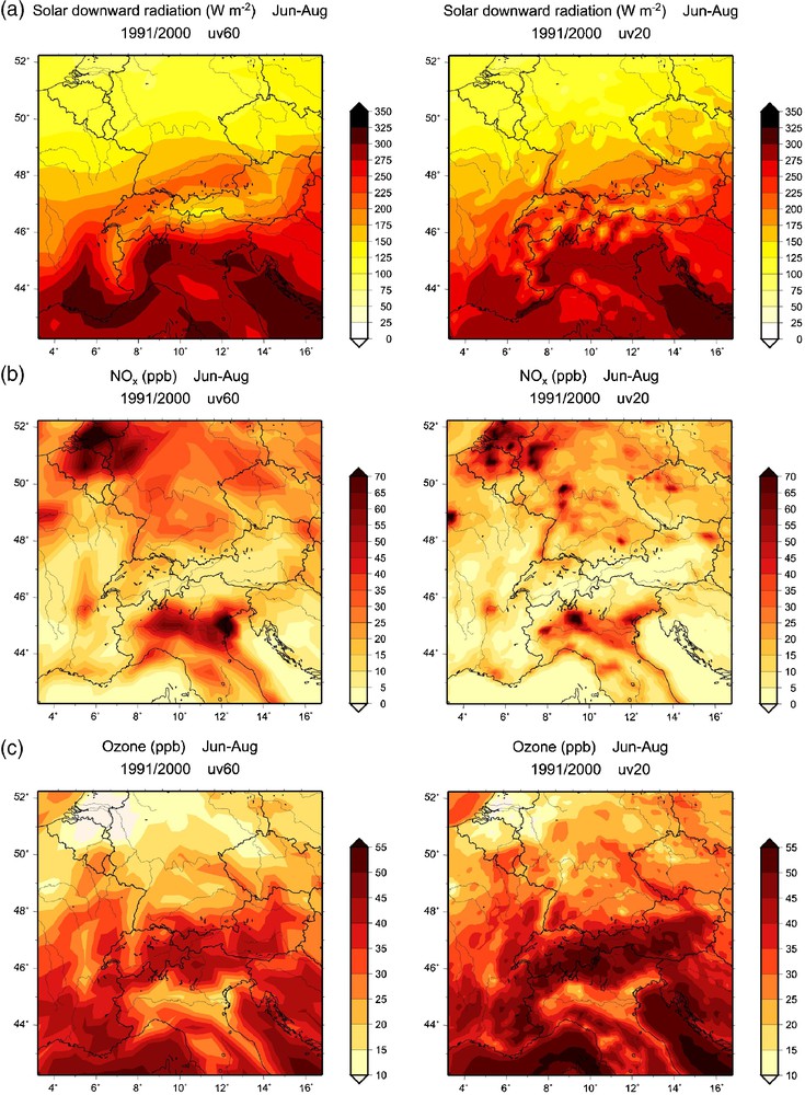
Simulated average values of downward solar radiation (a), NOx (b), and ozone (c) near the ground during summertime (June–August) for the time slice 1991–2000. The left column shows a clipping of Domain D1, the right column shows domain D2.
Fig. 2. Valeurs moyennes simulées du rayonnement solaire descendant (a), de NOx (b) et de l’ozone (c) près du sol pendant l’été (juin à août) pour la tranche de temps 1991–2000. La colonne de gauche montre un écrêtement du domaine D1, la colonne de droite montre celui du domaine D2.
As solar radiation is a necessary prerequisite for the formation of tropospheric ozone, the downward shortwave radiation is shown in Fig. 2a. The pattern of the incoming shortwave radiation is almost solely controlled by the distribution of cloud water content that has its highest values in the North and above mountain ranges (not shown). The differences between the patterns of the vertically integrated cloud-water content for the two resolutions can almost solely be attributed to the better representation in topography (see Fig. 1). Consequently, this pattern is also reflected in the shown distributions of the incoming shortwave radiation, which shows relative minima above mountaintops. The lower values in the northern regions found for both resolutions can also be attributed to higher cloud-water content for the considered summer months. Part of the bias can be attributed to the shortcomings of the regional model mentioned before, but it also cannot be excluded that uncertainties in the global simulation contribute to the overestimation of cloud cover.
The spatial distributions of the mean NOx (Fig. 2b) mixing ratios reflect almost completely the distributions of the anthropogenic NOx sources for 60- and 20-km resolutions, respectively. Since single source regions for NOx, such as Vienna, Munich, or Prague, are better distinguished for the fine resolution, simulated average ozone concentrations (Fig. 2c) are depressed in these urban centres due to titration effects. Simulated spatial patterns for D2 as well as the absolute values of the mean mixing ratios of ozone and NOx were found to agree rather well for the region of Bavaria [6]. However, for the regions with strong NO sources in the northwestern part of the investigation area, too high NOx and too low ozone mixing ratios are simulated. For example, for D2 the average value of simulated near-surface ozone for the region of North Rhine Westphalia was only 17 pbb, which is about 10 ppb too low as compared to observed average values. This underprediction of near-surface ozone can be attributed to an underestimation of meteorological situations favourable for high ozone concentrations, which is indicated by too low simulated solar radiation and, therefore, also in too low daytime boundary layer heights. The latter partly explains the too high simulated average NOx mixing ratios, which additionally result in too strong titration of ozone.
In agreement with the observations, daily mean ozone concentrations are higher on mountain sites than for urban regions due to the absence of a nocturnal decrease of the concentration. Since topography is smoothed at coarse resolutions, this effect is more pronounced in D2 than in D1 for the Alpine region and does not show up for smaller mountain ranges, such as the Vosges or the Black Forest, at a resolution of 60 km. Furthermore, the different representation of anthropogenic precursor sources and coastlines can result in pronounced resolution effects. For example, large differences between 60- and 20-km resolutions are found for the Po valley, in northern Italy. For the Milan region, the lower and broader NOx maximum at 60-km resolution can be clearly attributed to the smoothing of the source distributions for 60 km. Of course, this effect is also given for the Venice region. However, the simulated NOx for the Venice region is biased, due to the representation of the coastline, which is only coarsely resolved for the 60-km grid width. Therefore, the grid point including Venice is considered as water surface in the meteorological part of the model. However, part of the grid point's area includes anthropogenic emissions originating from the land fraction of the grid area. Due to the lower vertical exchange over the water during daytime, the emitted NO remains near the surface, which results in the high simulated surface NOx at this grid point, which directly affects near-surface ozone due to titration effects.
The scatter plots in Fig. 3 include NOx and ozone over Bavaria (observations for 1996–2000 from the Bavarian LfU network [1]) and NO2 and ozone at different sites in central Europe (observations form the EMEP network [4]). While most of the LfU stations are located in urban areas with high NOx concentrations and comparatively low average ozone, the stations of the EMEP network are located at remote sites and high altitudes. The scatter plots clarify that agreement between observed and simulated values is less good for D1 than for D2, since urban NOx source regions and mountain sites are hardly resolved for a resolution of 60 km. However, as mountains are still flattened at a resolution of 20 km, the observed high ozone mixing ratios found at distinct mountain sites are not fully reproduced by the simulation. The correlation coefficients for the mean ozone-mixing ratio given in Fig. 3 are in line with the correlation coefficients determined in other studies. Wild and Prather [45] found correlation coefficients of 0.566–0.578 for the Pacific area for resolutions T21–T106, whereas Langner et al. [28] found a correlation coefficient of 0.69 for Europe for a simulation with 0.8° resolution.
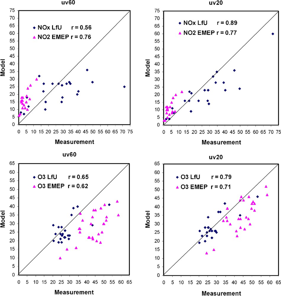
Scatter plots of model results for 60-km (left) and 20-km (right) resolutions versus observed values of summertime averages of near surface NOx and ozone in Bavaria from the LfU stations and of NO2 and ozone in Europe from the EMEP stations.
Fig. 3. Dispersion des points du modèle pour la résolution de 60 km (à gauche) et de 20 km (à droite), en fonction des valeurs observées pour les moyennes de l’été de NOx et d’ozone de surface en Bavière à partir des stations LfU et de NO2, et d’ozone en Europe à partir des stations EMEP.
3.2 Grid resolution impact on simulated climate change effects
The occurrence of high summertime concentrations of tropospheric ozone and other photooxidants is strongly determined by the meteorological conditions, in particular by the cloud cover, and by the lengths of clear sky episodes. Fig. 4 shows the simulated differences between present-day and future climate conditions for cloud water content and downward shortwave radiation along with the change of the emission of isoprene during summer (June–August). Even though the overall patterns are largely consistent for the two resolutions, the distributions of the meteorological variables as well as the chemical constituents show more distinct structures for domain D2 than for D1, due to the better resolution of topography and emissions.
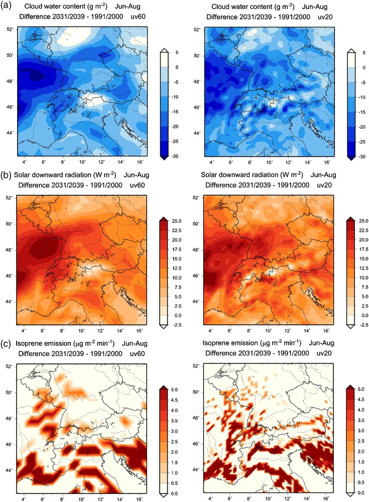
Differences between the simulated values of (a) vertically integrated cloud water content, (b) downward solar radiation, and (c) isoprene emission for present-day and future climate conditions during the months June–August. The left column shows a clipping of domain D1, the right column shows domain D2.
Fig. 4. Différences entre les valeurs simulées de la teneur en eau de nuages verticalement intégrée (a), du rayonnement solaire descendant (b) et de l’émission d’isoprène (c) pour les conditions climatiques actuelles et futures, au cours de la période juin–août. La colonne de gauche montre un écrêtement du domaine D1, la colonne de droite montre un écrêtement du domaine D2.
For the considered climate scenario, the cloud-water content decreases considerably between the 1990s the 2030s. Further analysis has shown that this decrease of the mean cloud water content can be attributed to an increase of the number of days without cloud cover. Analysis of the number of consecutive days with little or no cloud cover and of pressure tendencies [6] indicates that the decrease of the mean cloud water content can be attributed to a slight increase in the duration and frequency of anticyclonic conditions.
The decrease in cloudiness results in a corresponding increase of the incoming solar radiation. For the regions with maximum increase in incoming solar radiation, this corresponds to a relative change by almost 20%. The patterns in the change in shortwave radiation are almost identical with the change of the NO2 photolysis frequency, which is one of the most important photolysis frequencies for tropospheric photochemistry. Temperature (not shown) increases by 1.7–2.4 degrees, with the highest increase over central and southern France and the Po valley in northern Italy.
The emission of isoprene, which is the biogenically emitted compound with the highest ozone formation potential among the biogenic VOC, depends strongly on solar radiation and temperature. Therefore, higher isoprene emissions are simulated for future climate conditions. The spatial distribution of the change in isoprene emissions due to increased solar radiation and temperature is superposed by the distribution of forest areas that are high isoprene emitters. Consequently, the increase of the isoprene emission shows a patchy pattern that reflects strongly the representation of the distribution of isoprene-emitting plants in the model for the two grid-different resolutions. A maximum increase, corresponding to 30–50% of the emission for the baseline case, was found for the Black Forest, the Vosges, in southern France, former Yugoslavia, and for the forested regions in the Alps and the Apennine. Major differences between the results for 60 km and 20 km resolution show up in particular in eastern France and the western part of Germany, where patches covered with isoprene emitters are artificially spread for the 60-km resolution.
The resulting changes in mean daily ozone mixing ratios near the surface, the number of days with exceedance of the 60 ppb threshold for the 8-hourly mean during summer, and the April–September AOT40 (accumulated exposure over a threshold of 40 ppb during daytime) are shown in Figs. 5–7, together with the simulated values for the baseline case. A comparison of the simulated threshold exceedances and AOT40 with observations [44] shows a good agreement of the regional distributions over Germany except that – congruently with the mean ozone concentrations discussed in Section 3.1 – the simulated values are too low in the northern part of Germany.
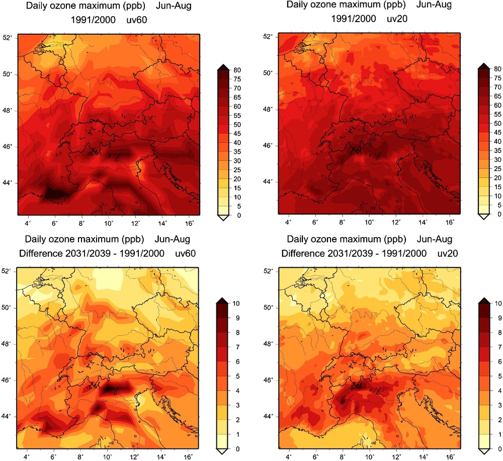
Simulated mean daily maximum of near surface ozone during the months June–August for present-day climate conditions (top) and differences between present-day and future conditions (bottom). The left column shows a clipping of domain D1, the right column shows domain D2.
Fig. 5. Maximum journalier moyen simulé de l’ozone de surface pendant les mois de juin à août pour les conditions climatiques actuelles (en haut) et différences entre les conditions actuelles et futures (en bas). La colonne de gauche indique un écrêtement du domaine D1, la colonne de droite montre celui du domaine D2.
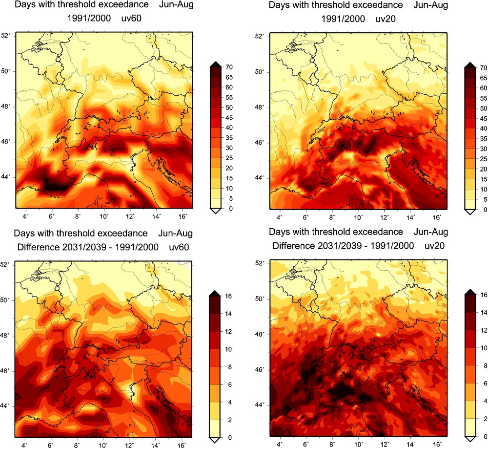
As Fig. 5 but for the number of days with exceedances of the threshold value of 60 ppb for the 8-h mean of near surface ozone during the months June–August.
Fig. 6. Idem Fig. 5, mais pour le nombre de jours présentant des dépassements de la valeur seuil de 60 ppb d’ozone de surface, pour une moyenne de 8 h pendant les mois de juin à août.
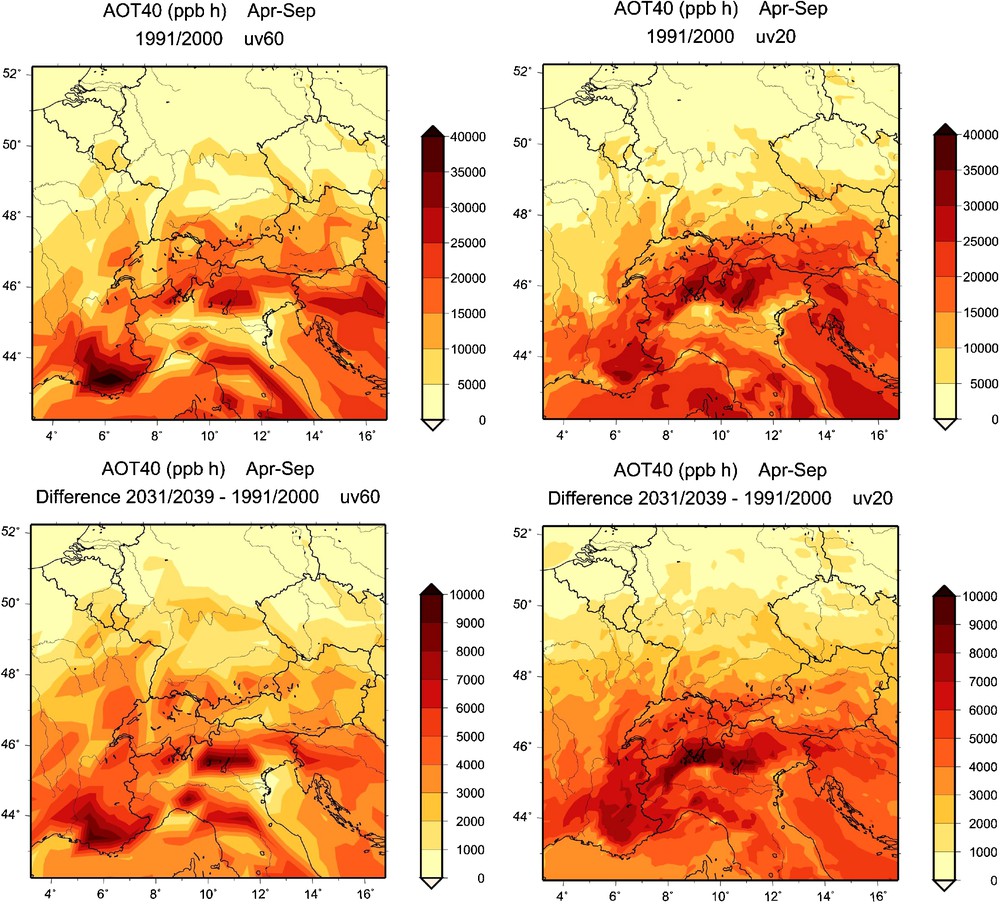
As Fig. 5, but for April–September AOT40.
Fig. 7. Idem Fig. 5, mais pour les données AOT 40 d’avril à septembre.
Comparison of the results for the 60-km and 20-km resolutions shows that the general tendencies in maximum ozone and critical levels are similar for both resolutions. However, strong regional differences can be identified as well. For example, the bias due to the coarse resolution of the coastline on the simulated near surface ozone for D1 influences also the simulated magnitude of the impact of climate change on near surface ozone in the Venice region.
At the first look, the highest increase of the maximum ozone concentration seems always to occur over areas with a strong increase of the isoprene emissions. This holds for both resolutions for southern France, northern Switzerland, or the region around Milan in northern Italy. A closer inspection of Fig. 5 together with Fig. 4c, and the NOx distributions in Fig. 2 shows that a high increase of the maximum ozone concentration is only found for those areas where a high increase of the isoprene emissions occurs together with high NOx mixing ratios. For example, the strong increase of the isoprene emissions over former Yugoslavia is not accompanied by a corresponding increase of near-surface ozone, since NOx is comparatively low (Fig. 2b). For the 20-km resolution, this holds also for the high-isoprene region at the border between Germany and Austria or the Black Forest. On the other hand, only the results for the 60-km resolution show a considerable maximum of the ozone increase north of the Main River. This feature can be explained by the fact that the high anthropogenic NOx emissions of the Frankfurt area are strongly smoothed and spread towards the northeast into an area with a high increase of isoprene emissions for the coarse resolution. For the resolution of 20 km, the regions where isoprene increases are spatially separated from the grid points with significant NOx emissions. Additionally, the increase in isoprene emissions is less strong for the 20-km resolution than for the 60-km one, as the maximum increase in solar downward radiation (Fig. 4b) is located farther towards the south.
According to the simulations, the target value of about 60 ppb for the 8-h mean of the ozone concentration will be exceeded on up to additional 15 days per summer for the future climate scenario (Fig. 6). As the 8-h mean of the near-surface ozone concentration is already closer to the threshold in mountain regions under present-day conditions, a stronger increase in the number of days with threshold exceedance occurs there. At these sites, a slight increase of the ozone concentration can result in a significant increase of the number of days with threshold exceedance. Due to the better representation of the topography, the pattern of this increase is more pronounced in the Alpine region and the Apennine Mountains for the 20-km resolution than for the 60-km. Further differences between the results for D1 and D2 occur also for polluted areas in southern Europe (e.g., Po Valley, Marseilles region).
The simulated change in April–September AOT40 for the considered area ranges between less than 1000 ppb h, for the northern part of Germany and the Benelux, up to more than 10 000 ppb h for some polluted regions in southern Europe. Compared to the sensitivity of the increase of the mean daily ozone maximum and of the number of days with threshold exceedance, the increase of the AOT40 index seems to be slightly less sensitive to grid resolution (Fig. 7).
4 Conclusions
Online coupled regional climate–chemistry simulations were carried out for two nested regions in Europe with horizontal resolutions of 60 km and 20 km. Climate-change effects on tropospheric ozone in central Europe were estimated by simulating about 10 years for the present-day and possible future climate conditions. The results for present-day conditions show reasonable agreement with observations. An exact reconstruction of the observed climate conditions can generally not be expected due to the internal variability of the climate system. Additional differences result from the shortcomings of the global and the regional model and from uncertainties with respect to the description of the Earth's surface and to the quantification of precursor emissions.
The simulations for future conditions are also affected by the assumed course of greenhouse gas concentrations. However, the choice of a particular scenario has no large impact on the results for the next decades as the scenarios diverge only slowly and due to the inertia of the climate system. For this study, the greenhouse gas scenario IS92a was used. The model results show how a climate change according to this scenario can affect the meteorological conditions and near-surface ozone within the next 30 years.
The nested simulations give a first impression how grid resolution can affect the results of regional climate–chemistry simulations for a given scenario. For both resolutions, the model results indicate that the future meteorological conditions in central Europe are more favourable to the formation of tropospheric ozone. Increased solar radiation due to decreased cloud cover, higher temperatures, and enhanced isoprene emissions promote the formation of tropospheric ozone and of other photooxidants. Biogenic emissions of isoprene had been found to increase regionally by up to 50%, because of higher incoming solar radiation for future climate conditions. For the case of unchanged anthropogenic precursor emissions, simulated daily maximum values of near-surface ozone mixing ratio increase by 10 ppb in northern Italy and 5–7 ppb for eastern France and southern Germany. Critical levels based on the exceedance of 60 ppb for the 8-h mean were found to increase by up to 16 days in summer and the April–September AOT40 was found to increase by up to 10 000 ppb h. Since the present results include only the effect of changed regional climate on near-surface ozone without considering changes in anthropogenic precursor emissions and land use, additional scenario studies are desirable for a complete picture.
General tendencies in maximum ozone and critical levels were found to be similar for the 60- and 20-km resolutions. However, pronounced differences between coarse and fine resolutions were found for several regions, due to smoothing of anthropogenic and biogenic emissions as well as flattened topography for the 60-km resolution. Although the effect of the over-dispersion of emissions for coarse grid resolutions on the results of regional air quality simulation was addressed in earlier investigations (e.g., [10,45]), it is important to clarify how this effect can bias the results of regional climate chemistry simulations for Europe.
The present study can be considered only as a first step towards a better understanding of the influence of grid resolution on the simulated results of regional climate change and its impact on near-surface ozone. The question of the appropriate resolution for a regional climate–chemistry study in relation to the topography and distribution of precursor emissions still needs more consideration. Further studies are desirable with an improved representation of sub-grid vegetation cover, for more recent global climate change scenarios, and for different grid resolutions. Open questions still exist on how far resolution-induced differences in simulated meteorological variables directly affect future regional distributions of near-surface ozone and which are the relative contributions of differently resolved isoprene emissions and anthropogenic emissions to the differences in the resulting ozone concentrations.
Nevertheless, the present results clearly indicate that regional interpretations of simulated changes in air quality due to changed regional climate must always be seen in the context of the grid resolution used for the simulations.
Acknowledgments
This investigation was funded by the Bavarian Ministry for Environment, Health, and Consumer Protection within the joint project BayForUV. The global climate simulations with ECHAM4 were supplied by the DKRZ (Deutsches Klimarechenzentrum) and the Max Planck Institute for Meteorology in Hamburg. Anthropogenic emission data were supplied by IER, University of Stuttgart. The simulations were carried out on three double-processor AMD 1900+ PCs with LINUX operating system. The authors are particularly indebted to E. Haas and J. Werhahn, who ensured the permanent availability of the computers.