Mobile bank conditions for laminar microrivers

Olivier Devauchelle; Christophe Josserand; Pierre-Yves Lagrée; Stéphane Zaleski

doi:10.1016/j.crte.2008.07.010

Surface Geosciences (hydrology-hydrogeology)

Mobile bank conditions for laminar microrivers
[Condition de berge mobile pour une rivière expérimentale laminaire]

Présenté par : Ghislain de Marsily

Olivier Devauchelle ¹ ; Christophe Josserand ² ; Pierre-Yves Lagrée ² ; Stéphane Zaleski ²

¹ Institut de physique du globe de Paris, 4, avenue de Neptune, 94100 Saint-Maur-des-Fossés, France
² Institut Jean-Le-Rond-d’Alembert, université Pierre-et-Marie-Curie, 4, place Jussieu, 75252 Paris cedex 05, France

Comptes Rendus. Géoscience, Volume 340 (2008) no. 11, pp. 732-740.

Résumés

Anglais
Français

The present study aims to establish a simple mechanistic model for river bank erosion. Recent experiments demonstrate that small-scale laminar flumes can develop erosion structures similar to those encountered in Nature. From the Saint-Venant Equations, a classical sediment transport law and a simple avalanche model, it is shown that bank failure caused by flow erosion can be represented through simple boundary conditions. These conditions are able to deal with the water level adjustment imposed by a constant water outflow condition. Finally, they are implemented to approach numerically the widening of a laminar river.

La présente étude se donne pour objectif d’établir un modèle simple de berge érodable. De récentes contributions ont démontré expérimentalement que dans des microrivières de laboratoire, parcourues par un écoulement laminaire, l’érosion peut produire des structures similaires à celles observées en milieu naturel. Les équations de Saint-Venant, en régime laminaire, associées à une loi de transport sédimentaire classique ainsi qu’à un modèle simplifié d’avalanche, permettent de déterminer un ensemble de conditions aux limites décrivant l’effondrement des berges sous l’effet de l’érosion et capables de prendre en compte des variations du niveau de l’eau de l’écoulement. Cette dernière propriété est indispensable si l’on souhaite imposer le débit total de la rivière. Enfin, ces conditions sont mises en œuvre dans le cas d’une microrivière rectiligne qui s’élargit sous l’effet de l’érosion.

Métadonnées

Reçu le : 2008-02-29
Accepté le : 2008-07-21
Publié le : 2008-09-26

DOI : 10.1016/j.crte.2008.07.010

Keywords: Geomorphology, Sediment transport, Bank erosion, Analogue modelling, Braided rivers, River morphology, Bedload transport, Microscale experiment
Mot clés : Géomorphologie, Transport de sédiments, Érosion des berges, Expérimentation analogique, Rivières en tresses, Morphologie fluviale, Charriage, Microrivières

Affiliations des auteurs :

Olivier Devauchelle ¹ ; Christophe Josserand ² ; Pierre-Yves Lagrée ² ; Stéphane Zaleski ²

@article{CRGEOS_2008__340_11_732_0,
     author = {Olivier Devauchelle and Christophe Josserand and Pierre-Yves Lagr\'ee and St\'ephane Zaleski},
     title = {Mobile bank conditions for laminar microrivers},
     journal = {Comptes Rendus. G\'eoscience},
     pages = {732--740},
     publisher = {Elsevier},
     volume = {340},
     number = {11},
     year = {2008},
     doi = {10.1016/j.crte.2008.07.010},
     language = {en},
}

TY  - JOUR
AU  - Olivier Devauchelle
AU  - Christophe Josserand
AU  - Pierre-Yves Lagrée
AU  - Stéphane Zaleski
TI  - Mobile bank conditions for laminar microrivers
JO  - Comptes Rendus. Géoscience
PY  - 2008
SP  - 732
EP  - 740
VL  - 340
IS  - 11
PB  - Elsevier
DO  - 10.1016/j.crte.2008.07.010
LA  - en
ID  - CRGEOS_2008__340_11_732_0
ER  -

%0 Journal Article
%A Olivier Devauchelle
%A Christophe Josserand
%A Pierre-Yves Lagrée
%A Stéphane Zaleski
%T Mobile bank conditions for laminar microrivers
%J Comptes Rendus. Géoscience
%D 2008
%P 732-740
%V 340
%N 11
%I Elsevier
%R 10.1016/j.crte.2008.07.010
%G en
%F CRGEOS_2008__340_11_732_0

Olivier Devauchelle; Christophe Josserand; Pierre-Yves Lagrée; Stéphane Zaleski. Mobile bank conditions for laminar microrivers. Comptes Rendus. Géoscience, Volume 340 (2008) no. 11, pp. 732-740. doi : 10.1016/j.crte.2008.07.010. https://comptes-rendus.academie-sciences.fr/geoscience/articles/10.1016/j.crte.2008.07.010/

Version originale du texte intégral

1 Introduction

The Saint-Venant equations, when associated to a sediment transport law, are able to represent the formation of various river patterns as fluid-structure instabilities. The most obvious example is the development of alternate bars in a straight channel [5,15]. The same bar instability is also responsible, at first order, for the formation of braided patterns [13,30]. A close relationship between bar instability and meander formation has been suggested earlier, to such an extent that both phenomena were hardly distinguished in the first contributions [17,5,30]. However, to investigate this relationship quantitatively, one needs to add a crucial ingredient to the model, namely a bank erosion law.

Advances in this direction may be credited to [21] and [2]. Both contributions use a heuristic bank erosion law, according to which the normal velocity of the bank is a continuous function of the water velocity near the bank. This model allowed to reproduce accurately wavelength of meanders, and shed light on the “bend instability” mechanism [2]. However, this heuristic bank erosion law presents serious drawbacks. First, it has not yet been derived from a detailed physical model, and thus lacks theoretical support. Second, it does not conserve sediment mass. In addition, the mechanisms leading to bank recess (undermining, bank failure) differ from bank advance processes (deposition, vegetation growth, etc.). Thus a bank erosion law should necessarily be discontinuous as the bank velocity changes sign. Last, there is no reason to believe that this law is a function of the mean water velocity only. It is a priori a function of every other model quantities, say water depth or bank height at least.

Since the contributions of [21] and [2], few attempts to derive bank erosion laws have been made. Among them are the work of [23], and more recently [8,10]. The later succeeded in numerically implementing complex bank erosion laws designed to take various phenomena into account (bed degradation, lateral erosion, bank collapse). Although [12] demonstrate the ability of their two-dimensional model to reproduce river meandering, the complexity of bank erosion laws pleads for a simplified analysis in the case of straight rivers, where only the transverse coordinate remains. This configuration also presents its own interest: the question of river width selection has been the subject of abundant research [18,31,32]. As a consequence, laboratory experiments were performed, and provide straight-river widening data [19,20,25].

The present study aims to derive a one-dimensional erosion law for a laminar flume on non-cohesive granular material, by means of a simplified but mechanistic approach. Our motivation is based on recent works tending to demonstrate that laminar flows may generate erosion patterns comparable to those encountered in Nature. This is true for rivers [11,26,28,37], but also for submarine canyons [27]. The main advantage in considering laminar flows is experimental: experiments involving laminar flumes of centimetric width are much more easily performed than their turbulent counterparts. The typical Reynolds number of a microscale experimental flume remains below 500 [29], a value low enough to approximate the flow by a laminar velocity profile [26].

This low value of the Reynolds number prevents direct upscaling from experiments to the field. However, the natural geometric aspect ratio, as well as the Froude number, can be respected. In that case, the shallow-water equations used here differ from the classical turbulent ones only by the value of the Boussinesq coefficient and by the friction term [11]. This analogy explains the qualitative similarity between laminar microrivers and natural ones. Thus microscale flumes should be regarded as powerful tools for the investigation of some geomorphological mechanisms, even though upscaling should be performed with great care [28].

This paper is organized as follows: a first section is devoted to a general two-dimensional model for erosion by laminar flows. Then the simple case of a rectilinear river is studied. Its limitations are discussed, and motivate the bank model presented in the next section. Finally, bank conditions are numerically implemented to represent the widening of a laminar river at constant water discharge.

2 Two-dimensional laminar flow and erosion

2.1 The Saint-Venant equations for the flow

Experimental laminar flumes generally imply shallow flows. Their typical depth is about 5 mm, whereas their width and length are of the order of 10 cm and 1 m respectively [26]. Consequently, the effects of the vertical water velocity may be neglected. This leads to the shallow-water approximation. The laminar Saint-Venant equations result from the vertical integration of Navier-Stokes equations, under the assumption that a parabola fits the vertical velocity profile (Nusselt film). A Nusselt film remains stable only for a Reynolds number below 5/(4S) (S being the mean slope of the flume [39]). Consequently, above this value the laminar Saint-Venant equations fail.

Another limitation of the model is due to the formation of ripples on the bed [9]. Again, keeping the Reynolds number low enough allows the bed to remain flat during an experiment. Similarly, alternate bars may grow in the channel, and one has to reduce the aspect ratio of the channel to avoid this drawback [11,19].

We hereafter assume that the flow characteristic time is much smaller than the erosion time. This is a common hypothesis in geomorphology [30]. It allows to neglect the time derivative in the flow equations. Momentum balance then reads

\frac{6}{5} F^{2} (u \cdot \nabla) u = S e_{x} - \nabla η - S \frac{u}{d^{2}},

(1)

where u, F, S, η and d denote the vertically averaged water velocity, the Froude number, the mean slope of the plane, the water surface elevation and the flow depth, respectively. These quantities were made non-dimensional, by mean of the typical velocity

U

and the typical depth

H

. The Froude number is then

F = U / \sqrt{g H}

. The 6/5 coefficient on the left-hand side of this equation is the Boussinesq coefficient for a laminar flow. In the following, x and y are the mean flow direction and the transverse direction, respectively (see Fig. 1).

Fig. 1
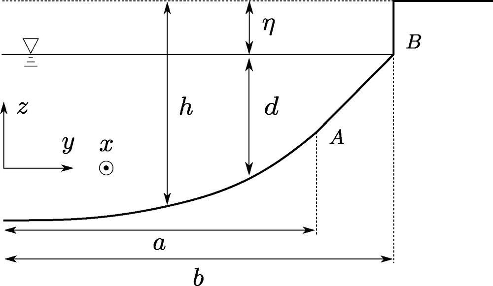
Simplified scheme of a microriver bank, and associated notations. By definition, avalanches occur only between point A and point B.
Schéma simplifié d’une berge de rivière expérimentale.

As for the momentum equations, the water mass conservation equation can be vertically integrated. This procedure leads to

\nabla \cdot (d u) = 0 .

(2)

From the solution of Eqs. (1) and (2), one can deduce the shear stress τ exerted by the stationnary flow: τ = u/d.

2.2 Sediment transport equations

2.2.1 The Exner equation

If the sediment particles are large and dense enough, their settling velocity is comparable to, or larger than, the water velocity. In that case, they remain at the river bed surface, and the flow transports them as bedload [6]. This mechanism is the dominant flow-induced transport in most experimental flumes, where suspension is negligible. Then, the bed topography evolution can be determined by means of the Exner equation [14]:

\partial_{t} h + \nabla \cdot q = 0,

(3)

where q denotes the horizontal sediment transport flux per unit length.

Bedload transport is induced by two forces: the tangential stress exerted by the flow, and gravity. A complete transport law should combine both effects [22,23]. However, for the sake of simplicity, we will hereafter separate these effects. We assume that the total sediment flux is the sum of an avalanche flux, independant from the flow, and an erosion flux induced by the shear stress τ. Then

q = q_{e} + \frac{1}{ε} q_{a},

(4)

where q_e and q_a denote the erosion and avalanche sediment fluxes, respectively. The small non-dimensional parameter ɛ indicates that avalanches occur at short time scales, as compared to erosion (see Section 2.2.3.).

2.2.2 Erosion by water

Numerous bedload models can be found in the literature [33]. It is usually considered that the intensity of the flux is a function ϕ of the Shields parameter θ:

∥ q_{e} ∥ = ϕ (θ),

(5)

where θ = ρν||τ||/(ρ_s − ρ)/d_s. The quantities ρ, ρ_s, ν and d_s denote water and sediment densities, water viscosity and the mean diameter of sediment grains. The shape of function ϕ itself is the subject of intense research (see [7] among others). It obviously vanishes at the origin on a flat bed. It is also generally accepted that it is a positive, growing and convex function. The main question about ϕ concerns the existence of a threshold, below which no grain moves. The analysis presented below (excepted the illustrative case of Section 3.1) holds for any erosion law ϕ. For illustrative purposes, we will set ϕ = θ^β with β = 3.75, as this empirical formulation fits correctly Charru and Heiff’s data [7], as well as the experiments of Malverti, Lajeunesse and Métivier [28]. Way above the threshold, most formulations tend to a power law. Of course, for a river slightly above the threshold, a more specific analysis would be required.

Regarding the direction of the sediment flux, we are not aware of any definitive model supported by experimental evidence, despite some recent important advances [16,23,36]. However, for moderate bottom slope, many authors suggest that the two-dimensional sediment flux may be expressed as follows:

q_{e} = ϕ (θ) (\frac{u}{∥ u ∥} - γ \nabla h),

(6)

γ is a constant (or a two-dimensional tensor) of order one [34,35,38]. The sediments are transported essentially along the water velocity direction (u/||u||). This direction is then corrected downwards by the bottom slope (γΔh).

2.2.3 Avalanches

A complete dynamical model for granular flows is far beyond the scope of the present study. In order to take the effects of avalanches into account, we use a simple heuristic model, proposed by [1].

In non-cohesive granular materials, avalanches are intermittent and local phenomena, occurring only if the surface slope exceeds a critical angle denoted α_c [3,4]. If we neglect the effect of inertia, the avalanche flux can be modelled by a growing function of the slope, vanishing below the threshold [24]:

q_{a} = φ (∥ \nabla h ∥) \frac{\nabla h}{∥ \nabla h ∥},

(7)

where φ vanishes below α_c.

Measuring the intensity of sediment transport by avalanches on a microscale river would not be an easy task. However, a rough order-of-magnitude analysis allows to compare avalanche transport to flow-induced transport. Both can be scaled by V_s/d², where V_s is the settling velocity [7]. During an avalanche, all the surface grains are driven by gravity, and thus are moving at velocities of the order of V_s. The associated flux is then of order V_s/d². On the other hand, erosion moves only a small fraction of the bed surface particles: for a Shields parameter equal to 0.3 (typical in laminar flumes), the erosion flux is less than 0.05V_s/d² [7]. Consequently, the small parameter ɛ introduced in Section 2.2.1 is of the order of 0.05.

In the general case, the system formed by the above equations cannot be solved easily, even numerically, due to the large time-scale separation between avalanches and erosion. Instead, one can take advantage of the small value of ɛ to derive integral conditions describing avalanches. It is the purpose of the following developments.

3 Laminar flume widening

3.1 A simple case: no avalanche and constant water level

In a first attempt to evaluate some solutions of the above erosion model, one may consider a straight river, without any avalanche. This simple case can be analytically solved as follows.

Since the flume cross-section is invariant with respect to any translation in the flow direction (that is, x), the full problem reduces to one-dimensional equations, where only y and t remain. The Saint-Venant Eqs. (1) and (2) then read θ = θ_*d and $θ_{*} = ρ g S H / (ρ_{s} - ρ) d_{s}$ . In the same way, the Exner equation becomes

\partial_{t} h = - \partial_{y} q, q = q_{e} + \frac{1}{ε} q_{a},

(8)

where the sediment fluxes are

q_{e} = - γ ϕ (θ_{*} d) \partial_{y} h,

(9)

q_{a} = - φ (| \partial_{y} h |) sign (\partial_{y} h) .

(10)

Note that q_e and q_a are transverse fluxes. Indeed, the sediment flux along the x-direction remains constant in a straight river, and thus does not influence its morphology.

If one assumes that no avalanche occurs, and if one represents the erosion function by a power-law (ϕ(θ) = θ^β), then a simple analytical solution can be derived [11]¹:

h = - \frac{1}{t^{1 / (β + 2)}} {(A - \frac{β y^{2}}{2 (β + 2) t^{2 / (β + 2)}})}^{1 / β},

(11)

where

A

is a constant linked to the river section area. This solution is valid only if η = 0 at any time.

This solution illustrates the limitations of a model without avalanches. Indeed, for β > 1 (this is usually the case in the literature), the bed transverse slope ∂_yh diverges at the bank (that is, for h = 0). For a non-cohesive sediment, such steepness triggers avalanches. Consequently, there must be a domain in the bank neighbourhood where avalanches occur. This idea inspired the bank model presented in the following section.

3.2 Non-cohesive bank conditions

3.2.1 Model description

A realistic non-cohesive bank model should describe the effect of avalanches that undermine the bank foot. It should also be able to take water level variations into account, so that the total water outflow Q can remain constant (see Section 3.3.1). The simplest way to do so is to assume that avalanches are contained at the bank foot, as on Fig. 1. We define a point A which x-coordinate is denoted by a:

\partial_{y} h \{\begin{array}{c} < α_{c} & on & [0, a) \\ \geq α_{c} & on & [a, b] \end{array}

(12)

The bank height is represented by a discontinuity of the topography h at point B (with coordinate b) where the flume depth vanishes. This assumption corresponds to experimental flumes behaviour. Indeed, above the water level, sediments are wet but unsaturated, and capillarity then introduces the cohesion required to maintain vertical banks.

Finally, for the sake of simplicity, the sediment topography out of the river bed is assumed to be uniform, and arbitrarily set to zero.

3.2.2 Boundary conditions

Boundary conditions at point A rest on the continuity of both bed topography and sediment flux. The first condition comes from the absence of cohesion in the fully saturated sediment, which cannot sustain an infinite slope. The second condition is imposed by the sediment-mass conservation. Thanks to the continuity of both h and q at point A (that is, for x = a(t)), one may write

h (a (t), t) = h_{-} (t),

(13)

q (a (t), t) = q_{-} (t),

(14)

where h_ and q_ denote the limit values of h and q at the left-hand side of point A. Both are functions of time only.

Point B is the intersection of the water surface with the topography, thus

h (b (t), t) = η .

(15)

The sediment mass conservation at point B requires that the flux be the product of the topography discontinuity with the horizontal velocity of the point B itself

q (b (t), t) = η \dot{b} .

(16)

Associated to these boundary conditions, Eqs. (8), (9), associated with (10) can be solved on segment [a,b], provided the boundary conditions q_ and h_ are fixed.

The following section is devoted to the derivation of bank conditions, based on the small value of ɛ. In Section 3.3, the derived equations are presented and solved.

3.2.3 Asymptotic analysis of the bank foot

3.2.3.1 Series expansion

To take advantage of the quick avalanche hypothesis (that is, ɛ is small), we will hereafter assume that the bank foot zone geometry is constrained by the first order of the sediment transport equation. In other words, the bed slope near a receding bank is close to the critical slope α_c. Order-one perturbations of this slope then control the sediment flux, even though they are geometrically negligible. Mathematically, these results are obtained by means of a perturbation analysis in ɛ.

The height of the river bed may be expanded as $h = h_{0} + ε h_{1} + O (ε^{2})$ . Similarly, let us define q_e,0 and q_e,1 for the erosion flux, q_a,0 and q_a,1 for the avalanche flux and b₀ and b₁ for the bank position². To zeroth order, the flux boundary condition (14) gives:

q_{a, 0} = 0, q_{e, 0} + q_{a, 1} = q_{-},

(17)

for y = a. In the same way, the boundary conditions (13), (15) and (16) lead respectively to:

h_{0} = h_{-}, h_{1} = 0 for y = a,

(18)

h_{0} |_{b_{0}} = η, h_{1} |_{b_{0}} + b_{1} (\partial_{y} h_{0}) |_{b_{0}} = 0,

(19)

q_{a, 0} | b_{0} = 0, η {\dot{b}}_{0} = q_{e, 0} |_{b_{0}} + q_{a, 1} |_{b_{0}} + b_{1} (\partial_{y} q_{a, 0}) |_{b_{0}} .

(20)

Finally, imposing the definition of point A (12) requires that

\partial_{y} h_{0} \geq α_{c}, \partial_{y} h_{1} \geq 0 .

(21)

3.2.3.2 First integration of the Exner equation

At order 1/ɛ, the Exner Eq. (8) reads

\partial_{y} q_{a, 0} = 0

(22)

for any y on [a,b]. Boundary conditions (17) and (20) then lead to q_a,0 = 0 on [a,b]. Now, the avalanche flux expression (10) leads to q_a,0 = −φ(∂_yh₀). Given the avalanche law φ and relation (21), one can impose a vanishing flux q_a,0 only by setting ∂_yh₀ = α_c. Finally, the topography profile at zeroth order is solved, taking the boundary condition (18) into account: h₀ = α_c(y − a) + h_. The boundary condition (19) at the bank foot then imposes the geometrical bank relation

α_{c} (b_{0} - a) = η - h_{-} .

(23)

3.2.3.3 Second integration

The bank relation (23) does not provide enough constraints. Fortunately, the next order of our expansion is easily reached. The Exner Eq. (8) imposes ∂_th₀ = −∂_yq_e,0−∂_yq_a,1. Taking the boundary condition (17) into account, this equation can be integrated into

q_{a, 1} = (y - a) (α_{c} \dot{a} - {\dot{h}}_{-}) - q_{e, 0} + q_{-},

(24)

keeping in mind that

\dot{a}

and

{\dot{h}}_{-}

are functions of time only. The flux boundary condition at the bank (20) imposes that

η {\dot{b}}_{0} = (b_{0} - a) (α_{c} \dot{a} - {\dot{h}}_{-}) + q_{-},

(25)

where the leading order of the Exner Eq. (22) has been used.

The next step requires the development of the sediment flux expressions (10) and (9) to order one and zero respectively:

q_{a, 1} = - \partial_{y} h_{1} φ^{'} (α_{c}),

(26)

q_{e, 0} = - γ α_{c} ϕ (θ_{*} (η - h_{0})) .

(27)

It is then possible to integrate Eq. (24) from a to any y. This provides an expression for the bed topography at order one:

h_{1} = - \frac{1}{φ^{'} (α_{c})} (\frac{1}{2} {(y - a)}^{2} (α_{c} \dot{a} - {\dot{h}}_{-}) + (y - a) q_{-} + \frac{γ}{θ_{*}} (Φ (θ_{*} (η - h_{-})) - Φ (θ_{*} (η - h_{0})))),

(28)

where Φ refers to the primitive of ϕ which vanishes when its argument does. An example of this order one perturbation is shown on Fig. 2. Finally, the remaining boundary condition (19) fixes the position b₁ of the bank foot at order one.

Fig. 2
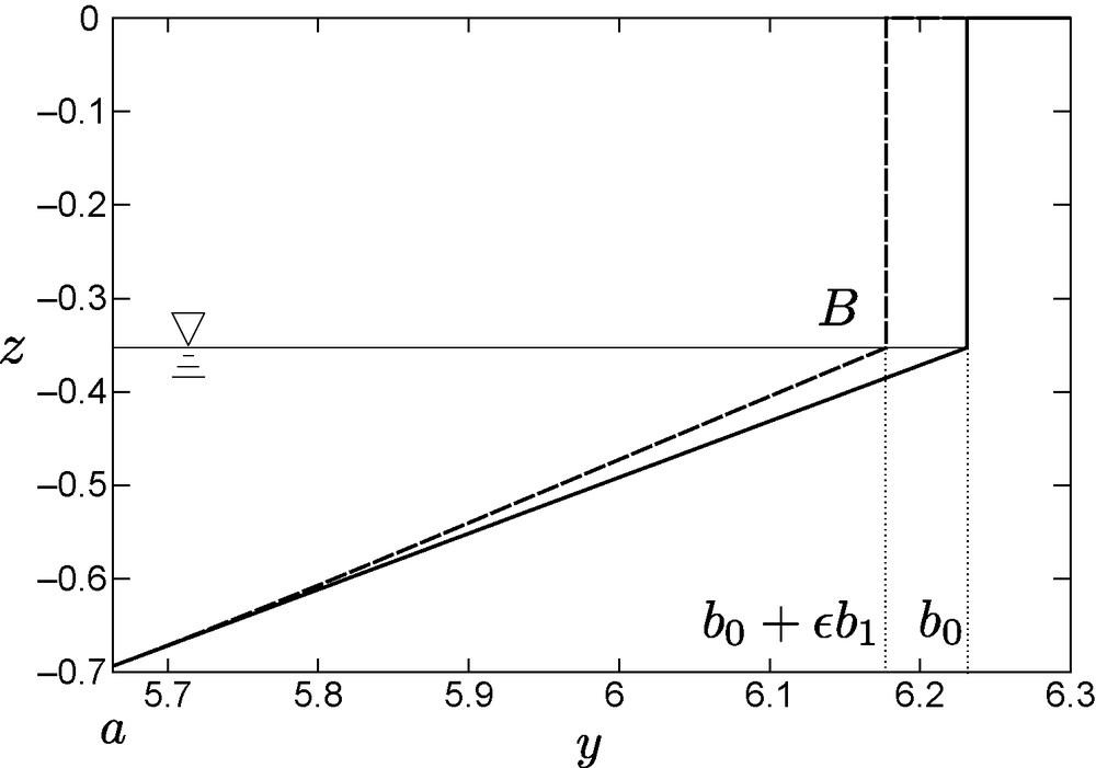
Example of the first-order development presented in Section 3.2.3. This picture corresponds to time t = 10 of the laminar river widening of Fig. 3. Solid line: h₀; dashed line: h₀ + ɛh₁. To enhance the effect of order one in the perturbation theory, ɛ is arbitrarily set to 10. In practice, the zeroth order is enough to derive the boundary condition for the bed evolution equations.
Développement à l’ordre un de la berge, selon le modèle présenté dans le paragraphe3.2.3.

3.2.3.4 Slope boundary condition

As long as the river widens, sediments are transported from the bank toward the bed, that is, $q_{-}$ ≤ 0. Since, by definition, no avalanche occurs on [0,a), $q_{-}$ is due to erosion only, and:

q_{-} = - γ ϕ (θ_{*} d_{-}) \partial_{y} h_{-}

(29)

Its minimum value is then $q_{-} \geq - γ ϕ (θ_{*} d_{-}) α_{c} = q_{e, 0} |_{a}$ . From boundary condition (17) we then deduce that q_a,1 ≥ 0, which can be satisfied only if q_a,1 = 0. In other words, the sediment flux due to avalanches vanishes at y = a. Consequently, relations (29) and (17) lead to the following boundary condition:

\partial_{y} h_{-} = α_{c} .

(30)

3.2.3.5 Self-consistency of the development

The bank model presented here requires that the topography slope ∂_yh remains above the avalanche angle on [a,b]. At order one, inequality (21) must be satisfied. Rewriting Eq. (24) by means of relation (26), the previous inequality reads $f (y) \equiv (y - a) (α_{c} \dot{a} - {\dot{h}}_{-}) - q_{e, 0} + q_{-} \leq 0$ . Indeed, whatever the avalanche law φ, the sediment flux increases with the topography slope, and thus the quantity φ′(α_c) is positive. We will see hereafter that f is indeed negative on [a,b₀], for some very general hypotheses on the sediment transport laws.

The second derivative of f reads $γ α_{c}^{3} {ϕ^{'}}^{'} (θ (η - h_{0})$ , and thus remains positive. Consequently, the first derivative f′ is a growing function. Its value in b₀ is $f^{'} (b_{0}) = α_{c} \dot{a} - {\dot{h}}_{-} - γ α_{c}^{2} ϕ^{'} (θ (η - h_{0}))$ We may assume that the derivative of the erosion law ϕ vanishes for a vanishing Shields parameter. Also, for wide rivers (see Section 3.3), $\dot{a} ≫ {\dot{h}}_{-}$ and f′(b₀) is positive.

The sign of f′ in a is not obvious. However, it will be shown below that the sign of f′ must change on [a,b₀], thus f′(a) must be negative.

Consequently, the variations of f are the following: f(a) = 0, then f decreases until it reaches a minimum, then increases up to $f (b_{0}) = η {\dot{b}}_{0}$ . For a widening river, ${\dot{b}}_{0}$ is positive, whereas η is negative. Thus f(b₀) remains negative, proving both that f′ must change sign as assumed above, and that f is negative on the whole segment [a,b₀].

3.3 Widening and overflow

3.3.1 Numerical results

The bank model derived in Section 3.2.3 allows us to impose a constant water outflow. Let Q be this outflow:

Q \equiv \int_{- \infty}^{\infty} u d d y \approx 2 \int_{0}^{a} {(η - h)}^{3} d y,

(31)

where we have neglected the small amount of water flowing near the bank, through the segment [a,b]. By imposing that Q remains constant while the river widens, we impose a condition that replaces the constant water level imposed in Section 3.1.

If we associate the water outflow condition (31) to the boundary conditions (30) and (25), we finally end up with the following system:

\{\begin{array}{c} \frac{\partial h}{\partial t} = - \frac{\partial q}{\partial y} \\ q = - γ_{n} ϕ (θ_{*} (η - h)) \frac{\partial h}{\partial y} \end{array}

(32)

\int_{0}^{a} {(η - h)}^{3} d y = Q_{w}, {\frac{\partial h}{\partial y}|}_{0} = 0,

(33)

{\frac{\partial h}{\partial y}|}_{a} = α_{c}, α_{c} {q|}_{a} = η \dot{η} - {(h \frac{\partial h}{\partial t})|}_{a} .

(34)

To obtain the above system, the first derivative of the relation h_ = h(a(t),t) has been used.

The solution of this system for a given initial condition can be approached numerically. We employed an explicit finite-difference scheme to produce the results presented on Fig. 3.

Fig. 3
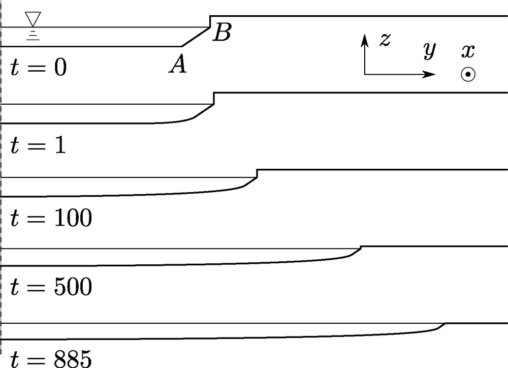
Widening of a straight microriver, at constant water outflow, using the bank conditions of Section 3.2.3. The spatial scale is arbitrary, but the aspect ratio is preserved. Parameter values are: θ_* = 1, α_c = 0.6, ϕ(θ) = θ^3.75, φ′(α_c) = 1. The initial section of the river is a rectangle of width a = 5 and depth h = −1. The initial water level is η = −0.4. This level increases as the bed widens, until it reaches the bank height. If the sediment transport law ϕ has no threshold, water eventually overflows.
Élargissement d’une rivière expérimentale laminaire, pour un débit d’eau constant. Larivière finit par déborder de son lit si le sédiment sur lequel elle s’écoule n’est pascohésif.

Under the effect of erosion and slope-induced sediment diffusion, the laminar river widens and becomes shallower. Eventually, the water level reaches the bank top, and water overflows. At that point, our model fails.

3.3.2 Sediment mass and water outflow constraints

The river overflow described above can be understood in a simple way. Bank erosion tends to widen the bed. However, due to the invariance in the main flow (that is x) direction, the sediment-mass conservation imposes that the flume section area S be conserved. In other words,

S \approx C_{1} WH

(35)

is a constant, where $W$ and $H$ respectively stand for the typical width and height of the river. C₁ is a shape constant of order one. Thus widening implies shallowing.

The water outflow Q is also a constant, which may be approached by

Q \approx C_{2} W {(η + H)}^{3}

(36)

for a laminar flow (C₂ is a shape constant). To maintain the outflow to its initial value while the river height decreases, the water level must increase. From relations (35) and (36), we can express the water level as a function of the river width:

η \approx {(\frac{Q}{W C_{2}})}^{1 / 3} - \frac{S}{W C_{1}} .

(37)

In Fig. 4, the above expression is compared with the numerical solution of Fig. 3, after setting arbitrarily C₁ and C₂ to one. Even though the two curves differ significantly, the simplified expression (37) reproduces qualitatively the behaviour of the numerical solution. In particular, for a very large river ( $W ≫ 1$ ), Eq. (37) becomes $η \approx {(Q / W)}^{1 / 3} > 0$ , therefore predicting an overflow. The fact that the numerical solution does not keep a rectangular shape explains the difference between the two curves.

Fig. 4
Water level of a widening laminar river vs its bed width. Solid line: numerical solution (the same as in Fig. 3); dashed line: simplified relation (37). The conservation of sediment mass and water discharge explains the overflow.
Évolution du niveau de l’eau au cours de l’élargissement. Trait plein : solution numérique ; trait pointillé: Eq. (37).

4 Conclusion

Under well established conditions (experimental laminar flumes on non-cohesive sediment), simplified bank conditions can be established. These conditions respect the sediment mass conservation. They are derived from the basic mechanism that controls bank erosion. If the sediment transport law does not include any threshold, the river bed widens until water overflows.

The model presented in this study is limited to a specific system. However, the method used here is quite general, and can probably be adapted to different situations (cohesive banks, vegetation growth, etc.). In addition, it can easily be generalized in two horizontal dimensions, provided the curvature of the bank remains small as compared to the flow depth.

Straight river widening experiments are found in the literature, but most contributions focus on the equilibrium width. Also, to our knowledge, no experiments were performed at low Reynolds number. Measurements on a laminar straight river are presently being performed at the Institut de physique du globe in Paris. Their comparison with the results presented in this paper is the subject of future work.

Acknowledgements

It is our pleasure to thank Daniel Lhuillier, François Métivier, Éric Lajeunesse, Luce Malverti, Antoine Fourrière, Bruno Andreotti and Philippe Claudin for seminal discussions. We also wish to thank the referees Christophe Ancey, François Charru and Philip Hall, as well as the editor Ghislain de Marsily, for their usefull advice.

¹ There is a typo in the relation (22) of [11]. The correct equation is given here.

² Developing b and not a is an arbitrary choice (the reverse would lead to the same results), since the only physically meaningful quantity is the distance between a and b.

Bibliographie

[1] B. Andreotti; P. Claudin; S. Douady Selection of dune shapes and velocities. Part 2: A two-dimensional modelling, Eur. Phys. J. B (2002)

[2] P. Blondeaux; G. Seminara A unified bar-bend theory of river meanders, J. Fluid Mech., Volume 157 (1985), pp. 449-470

[3] J.P. Bouchaud; M.E. Cates; J.R. Prakash; S.F. Edwards A model for the dynamics of sandpile surfaces, J. de Physique I, Volume 4 (1994), pp. 1383-1410

[4] T. Boutreux; E. Raphaël; P.-G. de Gennes Surface flows of granular materials: A modified picture for thick avalanches, Phys. Rev., Volume 58 (1998) no. 4, pp. 4692-4700

[5] R.A. Callander Instability and river channels, J. Fluid Mech., Volume 36 (1969) no. 3, pp. 465-480

[6] Chanson, H. The hydraulics of open channel flow: an introduction, Elsevier, 2004, pp. 141–241 (chapter 6).

[7] F. Charru; H. Mouilleron; O. Eiff Erosion and deposition of particles on a bed sheared by a viscous flow, J. Fluid Mech., Volume 519 (2004), pp. 55-80

[8] D. Chen; J.G. Duan Modeling width adjustment in meandering channels, J. Hydrol., Volume 321 (2006) no. 1–4, pp. 59-76

[9] S.E. Coleman; B.W. Melville Initiations of bed forms on a flat sand bed, J. Hydraul. Eng., Volume 122 (1996) no. 6, pp. 301-310

[10] S.E. Darby; A.M. Alabyan; M.J. Van de Wiel Numerical simulation of bank erosion and channel migration in meandering rivers, Water Resour. Res., Volume 38 (2002) no. 9, p. 1163

[11] O. Devauchelle; C. Josserand; P.-Y. Lagrée; S. Zaleski Morphodynamic modeling of erodible laminar channels, Phys. Rev. E, Volume 76 (2007), p. 05631

[12] G.D. Duan; P.Y. Julien Numerical simulation of the inception of channel meandering, Earth Surf. Processes, Volume 30 (2005), pp. 1093-1110

[13] F. Engelund; O. Skovgaard On the origin of meandering and braiding in alluvial streams, J. Fluid Mech., Volume 57 (1973) no. 2, pp. 289-302

[14] F.M. Exner Über die Wechselwirkung zwischen Wasser und Geschiebe in Flüssen, Sitzber. Akad. Wiss Wien (1925) no. 134 (In German)

[15] B. Federici; G. Seminara On the convective nature of bar instability, J. Fluid Mech., Volume 487 (2003), pp. 125-145

[16] S. Francalanci; L. Solari Gravitational effects on bedload transport at low Shields stress: experimental observations, Water Resour. Res. (2007) no. 43

[17] J. Fredsøe Meandering and braiding of rivers, J. Fluid Mech., Volume 84 (1978) no. 4, pp. 609-624

[18] R.E. Glover; Q.L. Florey Stable channel profiles., U.S. Bur. Reclamation Hydr., Volume 325 (1951)

[19] S. Ikeda Self-formed straight channels in sandy beds, J. Hydraul. Eng., Volume 107 (1981), pp. 389-406

[20] S. Ikeda; G. Parker; Y. Kimura Stable width and depth of straight gravel rivers with heterogeneous bed materials, Water Resour. Res., Volume 24 (1988) no. 5, pp. 713-722

[21] S. Ikeda; G. Parker; K. Saway Bend theory of river meanders. Part 1. Linear development, J. Fluid Mech., Volume 112 (1981), pp. 363-377

[22] C. Josserand; P.-Y. Lagrée; D. Lhuillier Stationary shear flows of dense granular materials: a tentative continuum modelling, Eur. Phys. J., Volume 14 (2004) no. 2, pp. 127-135

[23] A. Kovacs; G. Parker A new vectorial bedload formulation and its application to the time evolution of straight river channels, J. Fluid Mech., Volume 267 (1994), pp. 153-183

[24] T. Loiseleux; P. Gondret; M. Rabaud; D. Doppler Onset of erosion and avalanche for an inclined granular bed sheared by a continuous laminar flow, Phys. Fluids, Volume 17 (2005), p. 103304

[25] G.H. Macky Large flume experiments on the stable straight gravel bed channel, Water Resour. Res., Volume 35 (1999) no. 8

[26] L. Malverti, É. Lajeunesse, F. Métivier, Small is beautiful: upscaling from microscale laminar to natural turbulent rivers. J. Geophy. Res., 2008. In press.

[27] F. Métivier; E. Lajeunesse; M.C. Cacas Submarine Canyons in the Bathtub, J. Sediment. Res., Volume 75 (2005) no. 1, pp. 6-11

[28] F. Métivier; P. Meunier Input and output mass flux correlations in an experimental braided stream. Implications on the dynamics of bed load transport, J. Hydrol., Volume 271 (2003), pp. 22-38

[29] P. Meunier; F. Métivier Permanent transport regime of an experimental braided river. C. R. Acad., Sci., Paris Ser. IIA, Volume 331 (2000) no. 2, pp. 105-110

[30] G. Parker On the cause and characteristic scales of meandering and braiding in rivers, J. Fluid Mech., Volume 76 (1976) no. 3, pp. 457-480

[31] G. Parker Self-formed straight rivers with equilibrium banks and mobile bed. Part 2. The gravel river, J. Fluid Mech., Volume 89 (1978), pp. 127-146

[32] J.E. Pizzuto Numerical simulation of gravel river widening, Water Resour. Res., Volume 26 (1990) no. 9, pp. 1971-1980

[33] A.J. Raudkivi Loose Boundary Hydraulics, Pergamon Press, 1990

[34] R. Schielen; A. Doelman; H.E. de Swart On the nonlinear dynamics of free bars in straight channels, J. Fluid Mech., Volume 252 (1993), pp. 325-356

[35] M. Sekine; H. Kikkawa Mechanics of saltating grains, J. Hydraul. Eng., Volume 118 (1992), pp. 536-558

[36] G. Seminara; L. Solari; G. Parker Bed load at low Shields stress on arbitrarily sloping beds: Failure of the Bagnold hypothesis, Water Resour. Res., Volume 38 (2002) no. 11, p. 1249

[37] C.E. Smith Modeling high sinuosity meanders in a small flume, Geomorphology, Volume 25 (1998), pp. 19-30

[38] A.M. Talmon; N. Struiksma; M.C.L.M. van Mierlo Laboratory measurements of the direction of sediment transport on transverse alluvial-bed slopes, J. Hydraul. Res., Volume 33 (1995) no. 4, pp. 495-517

[39] C.-S. Yih Stability of liquid flow down an inclined plane, Phys. Fluids, Volume 6 (1963), pp. 321-334

Commentaires - Politique

Ces articles pourraient vous intéresser

The structure of powder snow avalanches

Betty Sovilla; Jim N. McElwaine; Michel Y. Louge

C. R. Phys (2015)

Modelling and simulation of powder-snow avalanches

Jocelyn Étienne; Marie Rastello; Emil J. Hopfinger

C. R. Méca (2006)

From a grain to avalanches: on the physics of granular surface flows

Stéphane Douady; Bruno Andreotti; Adrian Daerr; ...

C. R. Phys (2002)