

1 Introduction: from the Sun to the Earth's surface
The Earth is surrounded by a layer of relatively thin atmosphere whose density is exponentially decreasing with altitude. Most of the mass of the atmosphere, more than half, is concentrated in the first kilometres above the ground and 99.9% of it is concentrated below an altitude of 50 km. However, an atmosphere, holding several remarkable and vital properties, extends very far, up to several thousands of kilometres. In addition, the Earth is plunged into a solar and interplanetary environment and is finally imbedded in a magnetic shield, which plays a very important role in protecting the Earth both from the incoming energetic solar wind (Authier, 2002) and from the escape of atmospheric ions produced by the extreme ultraviolet solar radiation, a process, which in the case of Mars, has led to the quasi total loss of atmosphere (Fig. 1).
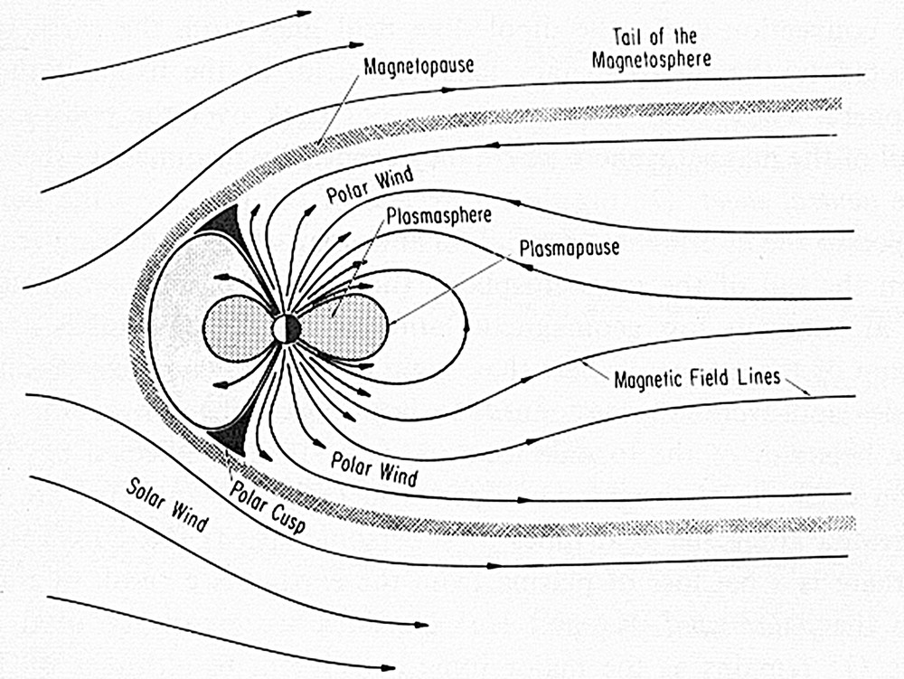
Schematic graph of the Earth's plasma magnetic environment where the various state parts of the magnetosphere are indicated with their names. According to Banks and Kockarts (1973), pp. 15.
Vue schématique de l’environnement magnétique du plasma terrestre. Les différentes parties de la magnétosphère sont indiquées avec leur nom. D’après Banks et Kockarts (1973), pp. 15.
This special issue is mainly devoted to the atmosphere of the Earth, which extends from the ground up to about an altitude of 85 km. This part represents the main contribution to the total air mass and is characterised, as concerns its major constituents (molecular nitrogen, molecular oxygen, argon, CO2), by a homogeneous chemical composition. The situation, however, evolves considerably further out, where, after a transition zone, from about 85 km up to 120 km, the atmosphere turns from the homosphere (constant chemical composition) to the heterosphere (light constituents, helium and hydrogen, becoming progressively with altitude, the major constituents) (Fig. 2). The transition from the homosphere to the heterosphere involves a competition between mixing and diffusive processes of constituents, while, in the same altitude range, the photodissociation of molecular oxygen by short wavelength solar radiation turns molecular oxygen into atomic oxygen. The question of diffusive separation of the different constituents is also strongly linked to turbulence (the source of mixing), which generally disappears at heights above about 100 km (Blamont and De Jager, 1961).
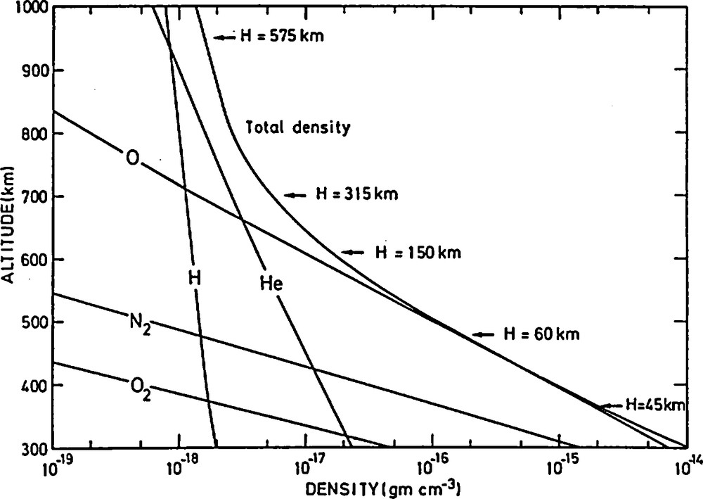
Variation of the density and scale heights H beyond 300 km in an terrestrial atmosphere with constant temperature (750 K). According to Banks and Kockarts (1973), pp. 15.
Variations de la densité et de l’échelle de hauteur au-delà de 300 km dans une atmosphère terrestre avec une température constante de 750 K. D’après Banks et Kockarts (1973), pp. 15.
In the heterosphere, each major constituent, molecular nitrogen, atomic oxygen, helium, hydrogen, is distributed as if it were alone: the greater the molecular (atomic) mass, the faster the decrease with respect to altitude. As a consequence, the average molecular mass decreases with altitude. The scale height H, characteristic of this exponential concentration decrease, increases with altitude (Fig. 2). In short, the distribution of the constituents evolves from a mixing to a diffusive process and, as a consequence, molecular nitrogen, atomic oxygen, helium and hydrogen are successively, with respect to altitude, the major constituents of the heterosphere (Barlier et al., 1978).
The thermal behaviour of the atmosphere (Fig. 3) reflects several physical processes of importance acting upon it. The troposphere, located just above the ground, is characterised by a negative temperature gradient resulting from the radiative balance of greenhouse gases and of convective processes. Above the tropopause, the stratosphere has a positive temperature gradient, induced by the absorption of solar radiation by the ozone layer. The mesosphere, above, has a negative temperature gradient due to the infrared emission of this layer. The mesophere is a region of decreasing temperature between the stratopause and the mesopause with a minimum of temperature (about 180 K) found at about 85 ± 5 km.
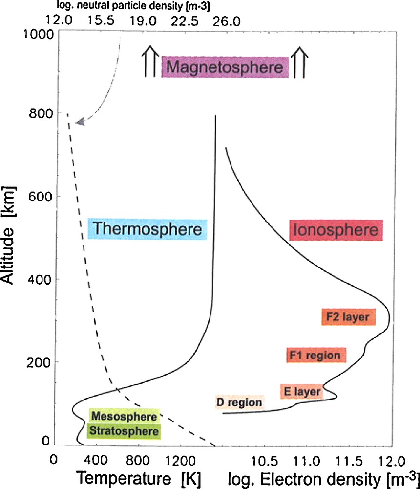
Vertical distribution of temperature in the homosphere and the heterosphere. Schematic graph of the ionosphere. According to Hagfors and Schlegel (2001), pp. 1560.
Distribution verticale de la température dans l’homosphère et dans l’hétérosphère. Diagramme schématique de l’ionosphère. D’après Hagfors and Schlegel (2001)Hagfors et Schlegel (2001), pp. 1560.
Above the mesosphere, the heterosphere (or thermosphere) is characterised by a strong positive temperature gradient. This temperature gradient is due to the absorption of short wave radiation from the Sun (photodissociation, photo-ionisation...), which are highly dependent upon solar activity: the temperature increases with altitude toward a limit (the exospheric temperature) of some 1000 K, which can almost double between minimum and maximum solar activity levels (Bruinsma et al., 2003). The upper part of the thermosphere, or exosphere, is characterized by mean free paths of atoms or molecules, which can exceed the scale height, allowing for some atoms to move into collisionless ballistic orbits under the influence of gravity. Some of the lightest atoms (hydrogen) can have velocities exceeding the escape velocity from the Earth and can be lost into space. The same situation should be encountered for high energy ions generated by the solar radiation, but the Earth's magnetic field confines them within the Earth environment: the magnetosphere.
The ionising properties of solar radiation have been indicated above; they lead to another feature of the upper layer of the atmosphere: the ionosphere. The electronic density progressively increases from about 50 km up to several hundred kilometres (Fig. 3). The electron density is layered with respect to altitude (labelled conventionally D, E, F1, F2). The formation of these layers can be understood on the basis of the atmospheric composition, of the absorption processes of short wavelength solar radiations and of collision processes (Risbeth and Garriott, 1969, Ratcliffe, 1972).
The pulse sounding technique initiated by the Americans Breit and Stuve was a basic tool in the knowledge of the ionosphere. Breit and Tuve in 1925 were both the discoverers of the ionosphere and the inventors of the ionosonde, in fact the first radar (Breit and Tuve, 1925). The discovery of the ionosphere revolutionized communication between people and became a major societal goal. The observation of the ionosphere mobilized from that epoch significant resources in order to develop scientific knowledge on the marine environment and on the propagation of waves in it. It was a unique means of telecommunication at the global scale. The knowledge of this very complex environment, even if communications at long range are nowadays provided extensively by other means including space technologies, remains an objective in itself and new societal goals have emerged in terms of the impact of the ionosphere on humans and systems in space and aeronautics on one hand, and on some major infrastructures such as electricity grids or pipelines on the other hand. As a consequence, a new activity, improperly named “space weather”, has developed in recent years in order to monitor and possibly to reduce the impact of ionospheric disturbances on human activities (aeronautics and space) and various systems.
Beyond the thermosphere and exosphere, there is the so-called plasmasphere, then what is called the magnetosphere (Ratcliffe, 1972). While the first Sputnik of the USSR discovered the lower layers of the upper atmosphere at several hundred kilometres of altitude, the first US satellite discovered the plasmasphere; this was Explorer-1 with an apogee of 2600 km height and a perigee of 370 km height, and it was launched on 1st February 1958. With a Geiger counter on board the counting of particles (protons and electrons mainly) increased beyond 1200 km instead of decreasing as a priori expected (see Fig. 6 for the precise shape of these belts, called the Van Allen belts, because Van Allen discovered them) (Hultqvist, 2001). Electrons and protons of high energy were trapped by the terrestrial magnetic field; the shape of these belts has been progressively better defined, thanks to different satellites. It is in fact important to mention the importance of the interaction of the Earth's magnetic field with particles coming from the Sun, i.e. the “solar wind”; the Earth's magnetic field is a dipole in the vicinity of the Earth; its main source is due to convection in the liquid core of the Earth (the terrestrial dynamo). But with this field, the solar wind particles (mostly protons and electrons) cannot usually penetrate into the atmosphere towards the Earth surface except by complex processes of interaction between the terrestrial magnetic field and the solar wind at high latitudes around 100 km altitude, giving rise, in particular, to the phenomenon of aurora. At the same time, the magnetic field lines are deeply deformed (Fig. 1). In this context, the Earth's magnetic field plays an important role as a shield. The magnetic shield is compressed towards the Sun side and takes on the contrary, the appearance of a comet tail on the opposite side. It extends to 10 Earth radii on the Sun side and up to 100 radii on the opposite side. Accordingly, the magnetosphere is a region difficult to observe and understand. To understand it, we must therefore make measurements simultaneously at multiple points in this space to capture all the processes involved in this magnetosphere; ESA launched in 2000, the Cluster-2 mission comprising four satellites with an altitude ranging between 4 and 19 Earth radii; the four satellites fly in formation in a tetrahedral shape. Finally, there are, beyond the magnetosphere, the Sun and the solar environment themselves, which can be very variable and not always predictable, with their own cycles of variability leading to significant effects on the terrestrial environment.
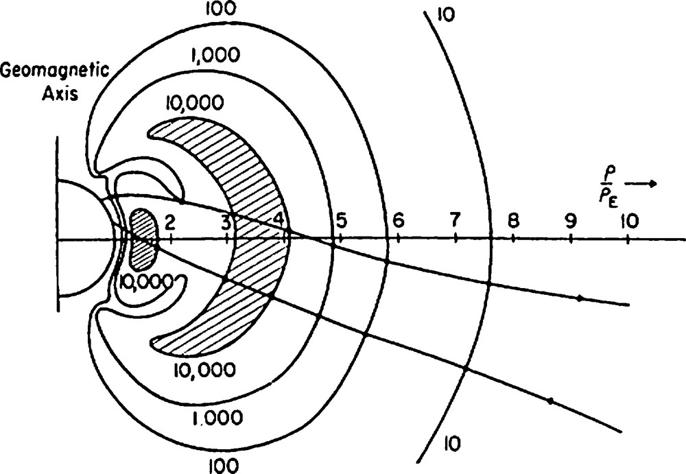
Van Allen belts. According to Hultqvist, 2001, pp. 1533.
Ceintures de Van Allen. D’après Hultqvist, 2001, pp. 1533.
At the opposite of these layers above the atmospheric 0–85 km layer, there is below the surface of the Earth, i.e. the sea and oceans and the solid surface of the Earth, i.e. the land and continents. There are also many interactions and exchanges among all these surfaces and the atmosphere (Trompette, 2003, pp. 273). The oceans cover 70% of the Earth's surface and represent an extremely large mass compared to that of the atmosphere; thus, the oceans have a great heat storage capability and exchanges with the atmosphere are very important. Oceans also have a great gas absorption capability from the atmosphere and a great gas emission capability towards the atmosphere, so many exchanges of constituents can occur. There is also a great capability for exchange of momenta with winds between the atmosphere and oceans. All these layers cannot be seriously studied ignoring these interactions.
It is of interest to remember that the ocean temperature is highly variable depending on seasons, latitudes, geographic locations. The same is true for many other parameters, such as albedo, especially in the polar regions if frozen or not, salinity, the state of the sea, waves, oceanic circulation at large and mesoscales. Reactions and consequences on the state of the atmosphere covering these surfaces are important. In conclusion, the knowledge of the atmosphere in its first layers, and as a result, weather forecasting, cannot be performed without taking into account all these interactions. This is the purpose of the operational oceanography centre, the Mercator Group located in Toulouse and which is a publicly funded group. This objective becomes essential.
In the solid part represented by the continents and land masses, one must distinguish the biosphere, the hydrosphere and the solid part, rocks and vegetal soils with their great diversity that cover the Earth's surface. The interactions and exchanges between the atmosphere and the different surfaces are also very important.
As an example, it may be recalled that between 540 and 240 million years ago, the atmosphere composition has changed profoundly under the influence of photosynthesis, which fixes the CO2, and the influence of the respiration of plants, which rejects oxygen. The rate of atmospheric CO2 was reduced by a factor of 10 while the oxygen doubled from 15% to around 30 to 35% (Nahon, 2008, page 112); this evolution has played a profound effect on the metabolism of organisms and on the biological evolution of our planet.
As another recent example, nowadays, a significant warming of the Earth is observed in the Arctic regions and as a result, the decrease of permafrost in northern Canada can be seen; the rate of thaw has tripled in last 40 years and the transition zone has moved by 30 cm per year to the north. This is true also in the Siberian region (Nahon, 2008, p. 144). Thus, one must take into account the expected role of gas emissions, such as CO2 and methane, in these regions with a possible burst and non-linear effects on the Earth's environment and atmosphere.
As a final example, we can still recall the role of volcanoes that emit gases and dust in the atmosphere, which may also significantly alter the climate.
In conclusion, we cannot understand the behaviour of the atmosphere and make long-term predictions of its evolution without taking into account many interactions, but that is obviously a delicate and difficult purpose to be performed and it is not easy to do.
2 General remarks on observatories and observations of the Earth's atmosphere in its first layers
2.1 Means for in situ technical measurements
The parameters of the Earth's atmosphere and its variations can be measured on the surface of the Earth (recording of meteorological parameters at ground level) and identically on the ocean surface (instruments on boats and buoys). However, as soon as one rises in altitude in situ measurements in atmospheric layers are increasingly more difficult to perform, and up to the mid-20th century, our knowledge was rather limited on these regions. Today, decisive progress has been made for a direct access to in situ measurements using new technologies, which are now completely operational (aircraft, balloons, rockets). Atmospheric parameter determination by remote sensing techniques has also been developed: active and passive instrumentations covering the whole electromagnetism spectrum from optical to radio waves (radiometers, radars, lidar, propagation characteristics...) from the ground or from observatories in space.
Let us first consider very briefly the possibilities offered by aircraft, balloons, and rockets.
2.1.1 Aircraft
In the first kilometres, an aircraft is a good vector for embarking scientific instruments. Standard aircraft can be used, and aircraft such as ATR-42 or F20 are effectively used. These aircraft have to be specially equipped with instruments dedicated to specific goals and dedicated campaigns. In France, Météo-France, Institut national des sciences de l’univers (INSU) and Centre national d’études spatiales (CNES), with the support of the Institut géographique national (IGN), have joined their efforts through the “SAFIRE” research service unit located in Toulouse in the framework of the MOZAIC programme. Next to such measurements, routine observations for meteorological and environmental applications can effectively take advantage of commercial aircrafts, specially equipped with dedicated instruments. These types of measurement, with automatic transmission in real time to the ground and weather centres, have been developed for routine monitoring in meteorology because of their relatively low cost compared to any other solution and continue to be used (Fig. 4). Measurements are made during the cruise of aircraft, i.e. most of the time at a single level (the level of flight at 10 km altitude); however near airports, observations can be made during the ascent and descent of aircraft. A larger quantity of data is thus obtained in the Northern Hemisphere than in the Southern Hemisphere as a function of the number of regular aircraft routes. It may be noted that aircraft can also be used to calibrate future space missions such as the mission of ESA, ADM-Eolus to be launched in October 2009 and primarily intended to measure winds by a lidar from space.
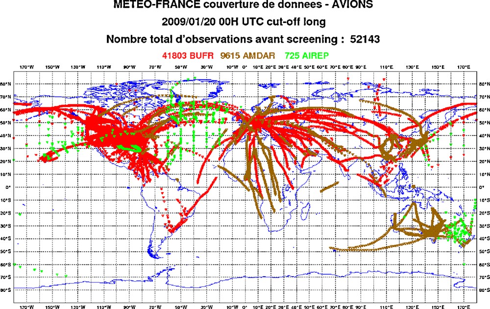
Covering of meteorological data by aircrafts for Météo-France on 20th January 2009. Colour corresponds to different networks and instruments. These are all observations available before the first operation performed by the assimilation called “screening” or “skimming” to eliminate some of the data, where they are too close together, so redundant. According to Pailleux, 2002 and photos produced by H. Bénichou, Météo-France in 2009.
Couverture des données météorologiques par des avions pour Météo-France le 20 janvier 2009. Les couleurs correspondent à différents réseaux et différents instruments. Ces observations sont disponibles avant l’opération dite d’écrémage pour éliminer les données trop proches les unes des autres et aussi redondantes. D’après Pailleux, 2002 et photos fournies par H. Bénichou, Météo-France en 2009.
2.1.2 Balloons
Beyond a certain altitude of about 10 or 15 km, the aircraft is generally not suitable for in situ measurements, but balloons can play a major role as well as at lower altitude with tropospheric balloons for meteorological purposes. The meteorological data (temperature, pressure, humidity, speed and force of winds) are performed within an international network twice a day (0 hour and 12 hours UTC), the global radiosonde network. The data are transmitted by radio (radiosonde). The elevation of these balloons can reach 35 km. The role of balloons is illustrated in Fig. 5.
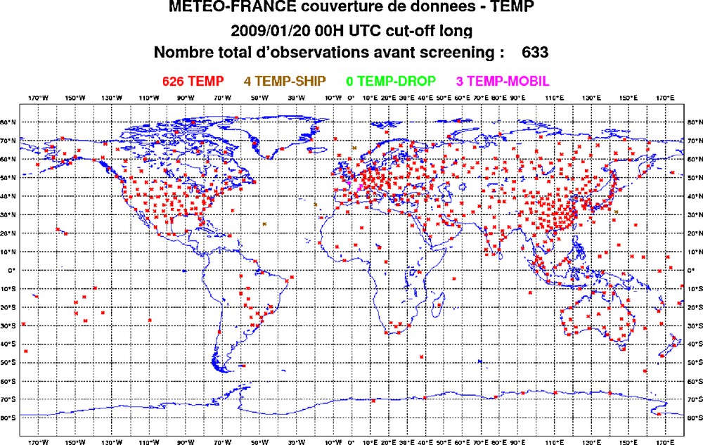
Temperature obtained by balloons on 20th January 2009 for meteorological purposes. Colour corresponds to different networks and instruments. According to Pailleux, 2002 and photos produced by H. Bénichou, Météo-France in 2009.
Temperature obtenue par ballons le 20 janvier 2009 pour des buts météorologiques. Les couleurs correspondent à différents réseaux et différents instruments. D’après Pailleux, 2002 et photos fournies par H. Bénichou, Météo-France en 2009.
Stratospheric balloons have also been developed. They can operate from 12 km and up to 45 km. The lifetime of certain types of balloon can reach a few months. There is a complex engineering for the realization of such balloons. The balloons are also used to test instruments to be installed onboard satellites.
2.1.3 Rockets
In an unfortunately tragic context, the Second World War showed that one could launch rockets that can reach very high altitudes, 100 km and far beyond, 200 km and more. The scientific use of rockets largely developed after the war, with many applications in astronomy (measurement of the solar spectrum at wavelengths impossible to collect from the ground) and in studies of the Earth's atmosphere. In this way, the knowledge of the physical and chemical properties of the atmosphere up to relatively high altitudes (a part of the atmosphere referred then, by some scientists, as “the ignorosphere”) was greatly improved (Blamont, 2001). However, the launch of a rocket turned out to be quite expensive for a very short experiment. The rocket was therefore not considered as suitable for a continuous and operational monitoring of the atmosphere. The idea of using artificial satellites carrying on board of instruments for in situ measurements or remote sensing techniques emerged during the 1950s at the time of the preparation of the International Geophysical Year (1957–1958). Satellites, due to atmospheric drag, can only operate above 200 km, which makes mandatory the use of remote sensing techniques for the observation of the “homosphere”.
2.1.4 Atmosphere under the sign of Space
2.1.4.1 Historical features
On 4th October 1957, the launch of the first artificial satellite by the Soviet Union in the framework of the International Geophysical Year caused a great shock in the media, political and even scientific world. Although such an event was advertised long in advance, its feasibility remained doubtful for many people. It is interesting to note that the only objective assigned to the satellite, in addition to transmitting its famous “Bip, bip” worldwide, was to gather information on the drag exerted by the atmosphere on this specifically spherically shaped satellite! The weight of Sputnik was 83 kg; its perigee (minimum altitude) was 225 km, its apogee (maximum altitude) 960 km, its period of 96 minutes and its expected life 3 months. The spacecraft crashed to Earth on 4th January 1958.
In the months that followed the launch of the first Soviet satellite, the Earth's flattening also was recomputed by geodesists with a much better accuracy than previously. In particular, significant systematic errors of the past determinations were exhibited. Inverting the air drag data led to estimate the atmospheric density of the upper atmosphere of Earth at the perigee altitude of Sputnik (about 200–300 km) showing significant differences with respect to the existing models. The extreme sensitivity of this density to the solar and geomagnetic activity was also demonstrated.
In a harsh competition, the USA launched Explorer I in February 1958 (1958 Alpha) weighing 14 kg. Explorer I was launched by the team of Von Braun thanks to a converted military missile. Apart from the Vanguard satellite launched on 17 March 1958 (1958 Beta), it was followed by Explorer III on 26 March 1958 (the second one failed) and by Explorer IV, launched on July 26 1958 (Rosso, 2001; Villain, 2003, 2007). These satellites, equipped with Geiger-Muller tubes for detecting energetic particle measurements, also permitted a remarkable breakthrough in the field of the atmospheric science: the discovery of the Van Allen belts using the detector onboard the satellites. These particles are naturally trapped in the magnetosphere (Fig. 6). This was actually one of the first major discoveries of the first space year.
Apart from the basic series of Meteosat satellites managed in Europe by EUMETSAT, an example of modern applications of space observation of the low atmosphere is given by the ESA mission, the ADM-Aeolus mission, scheduled for launch in 2010. The Atmospheric Dynamics Mission (ADM-Aeolus, 2010 http://www.esa.int/esaLP/LPadmaeolus.html) will provide global observations of three-dimensional wind fields. This space mission should help correct a major deficiency within the current meteorological observation network. ADM-Aeolus is intended to improve the accuracy of weather forecasting by providing data on winds and their variations, on the vertical distribution of clouds, the altitude of their upper limit and on the properties of aerosols using a Doppler Wind Lidar (DWL).
2.1.4.2 GPS
We give another example of the use of a space system for perennial societal applications to atmospheric sciences. The perennial property of GPS for navigation and positioning is fundamental for continuous scientific atmospheric applications. The global positioning system GPS is now a very efficient system for societal and routine scientific applications and especially in meteorology and in low atmosphere study. The interest of GPS in this field (Hajj et al., 2002; Barlier, 2008) should grow considerably. GPS receivers on board satellites in low orbit (purely meteorological satellites or missions of opportunity) can provide accurate information about the temperature profile in the stratosphere and upper troposphere and the humidity in the lower troposphere. This is the technique known as “radio occultation” in meteorology, which is able to exploit the radio signals emitted by GPS satellites, including Galileo satellites in the future, and Global Navigation Satellites Systems (GNSS) more generally (Barlier, 2008). When these signals, transmitted by the navigation satellites, pass through the Earth's atmosphere and are received by a low orbiting satellite, their speed of propagation is slowed down and they are refracted. The measurement of the integrated refractivity provides profiles of atmospheric refractivity from which can be obtained the relevant information on temperature, humidity (Hajj et al., 2002). Similarly, networks of ground based GNSS receivers yield maps of integrated water vapour. The interest of GNSS is that the system is now maintained independently of scientific applications due to the great importance of societal applications. In science, a great difficulty is often to migrate from experimental short-lived systems towards operational and permanent systems.
2.2 Some characteristics of Earth observations and observatories
2.2.1 The link between societal and scientific needs: GEO/GEOSS, GMES
The layer of the lower atmosphere 0 to 85 km has a fundamental scientific interest, but also has a large societal impact. This layer is vital for humanity in the most elementary sense. It is the air that is inhaled by humans, fauna and flora. In the context of the development of pollution and climatic changes, it has to be monitored in a continuous manner. Therefore, data on this layer must be obtained in a sustainable and continuous way. In terms of data acquisition and dissemination, the state of the art has considerably evolved in recent years through the use of space observations, of new information systems, of powerful computing facilities, of data transmission networks, of data archiving and of data accessibility.
In July 2003, the first World Summit on Earth Observation met in Washington. Governments adopted a declaration implying a political commitment to move towards developing a coherent, coordinated and sustainable system for Earth observations. The Summit established the first ad hoc intergovernmental Group of Earth Observations, GEO, in order to prepare a first 10 years implementation plan. After 2 years of work, the GEO was established on a permanent basis and a plan was set up to achieve a “System of Systems for Global Earth Observation”: Global Earth Observation System of Systems (GEOSS). GEOSS is intended to bring together all the countries of the world and encompass both in situ observations as well as airborne and space observations towards interdisciplinary research. The existing observation systems are the foundations of GEOSS. All observing systems participating in GEOSS keep their own mandate and mode of governance, but add their specific involvement in GEOSS (Baüer et al., 2006). In parallel for all these objectives and in fact as early as 1998 and before GEO, a programme was launched at the European level called Global Monitoring for Environment and Security (GMES). GMES is a European initiative for the implementation of information services dealing with environment and security (Baüer et al., 2006). By a combination of measurements at terrestrial level and from space, it rapidly became clear that new operational services could be offered in fields such as oceanography, precise mapping of land use, rapid mapping at times of emergency for the civil protection field or air quality monitoring. The progressive implementation of GMES is made possible by the activities and investments of European Union and ESA Member States.
2.2.2 Concept of Virtual Observatory: OV
Atmospheric data and information must be precisely controlled and validated. This involves comparisons and multiple sources as well as modelling and data assimilation. This also implies the implementation of modern information, computing, communication (Internet), data archiving and data access means. This is the basis of the concept of the virtual observatory. A virtual observatory is a network of interactive data archives and software tools which make use of the Internet to build a scientific research environment. The virtual observatory can automate the procedure, often difficult and painful, of researching and collecting geodetic and geophysical data, and cross-checking the information to create a whole greater than the sum of its parts. This is made possible through a considerable effort to standardize both, data and methods, and tools of the atmospheric community (scientists, users...).
2.2.3 Governance required
Access to data, control, validation, intercomparison and assimilation of data, as well as modelling, imply a high level of organisation and management and call for a “governance”. Such a governance, ensuring in real time interoperability and easy access to the data of very diverse origins, has, for a long time, been achieved by the international meteorology community through the World Meteorological Organisation (WMO). However, in many respects, a large effort has yet to be made to extend such a governance to the other aspects of atmospheric science and monitoring.
The volume of data to be considered is increasing, the complexity of these data as well. These data should also benefit from long time archiving, which is a major challenge. However, another difficulty arises from the frequent changes of media support available: informatic supports are often not compatible with each other and become obsolete with the disappearance of suitable technical supports. All this requires much effort and cost in terms of people, scientific and agencies, and international cooperation. Researchers and agencies are often reluctant to initiate, in order to address these challenges, endeavours, which may not be perceived to be as essential as they are rewarding.
Data accessible anywhere, at any time and for all users is another challenge. Internet is, as is well known, a powerful tool, but it generates a new problem of governance at national and international levels.
3 A glimpse at dense atmosphere neighbours: the thermosphere, oceans and land
Monitoring the dense atmosphere implies also the monitoring of its interactions with the Earth's surface and the upper atmosphere. Data on this sector must also be obtained in a sustainable and continuous manner. As an example, one cannot study CO2 evolution without considering, at the same time, the process of deforestation or reforestation, the degradation of the environment, the evolution of oceans… The data provided by, for example, the Landsat satellites, is essential (Houghton and Goetz, 2008). Other examples are provided by the study of ozone which necessitates the monitoring of the UV radiation incoming from the Sun (Baüer et al., 2006) and by the study of the increase of the mean sea level, which calls for investigating the global water cycle.
3.1 Thermosphere
The models of thermosphere density have an uncertainty of about 15 to 20%, partly due to a lack of relevant data. Improving knowledge of the Earth's atmosphere is a research area in its own right, and is useful for planning and monitoring satellite missions into low Earth orbit. Data on atmospheric density have been in the past regularly collected, archived and used to build thermosphere models such as DTM (Barlier et al., 1978). Recent missions, such as CHAMP (at 450 km in the beginning of the mission 2000–2008, up to 250 km at the end of the mission) and GRACE (launched at 480 km in the beginning of the mission in 2002), equipped with accelerometers give a direct access to the drag exerted by the atmosphere on the spacecrafts and therefore to the local atmospheric density. The STAR accelerometer on board the German satellite CHAMP allows the measurement of the forces acting on the satellite surface with a good accuracy (∼10-9 m/s2) and with a high spatio-temporal resolution. An analysis of the variations observed with CHAMP and GRACE has been made (Bruinsma et al., 2004; Menvielle et al., 2004). In the future, data from accelerometers mission GOCE (2009 at 250 km) and MICROSCOPE (to be launched in 2013 at 730 km) should usefully, through the sampling of the atmosphere at different altitudes, complement the database.
3.2 Examples of interaction between ocean and winds: El Niño and sea surface temperature
The climate is strongly determined by the interactions between the atmosphere and the ocean: the atmosphere triggers ocean phenomena through the actions of wind, precipitations and the transmitted solar radiation. The ocean responds by warming or cooling the atmosphere through the combined effects of heat transfer and ocean currents. Climate models are based on coupled atmospheric and ocean modelling, thus making ocean models essential for climate modelling. Fig. 7 gives an example of forecasting of sea surface temperature in the Atlantic Ocean.
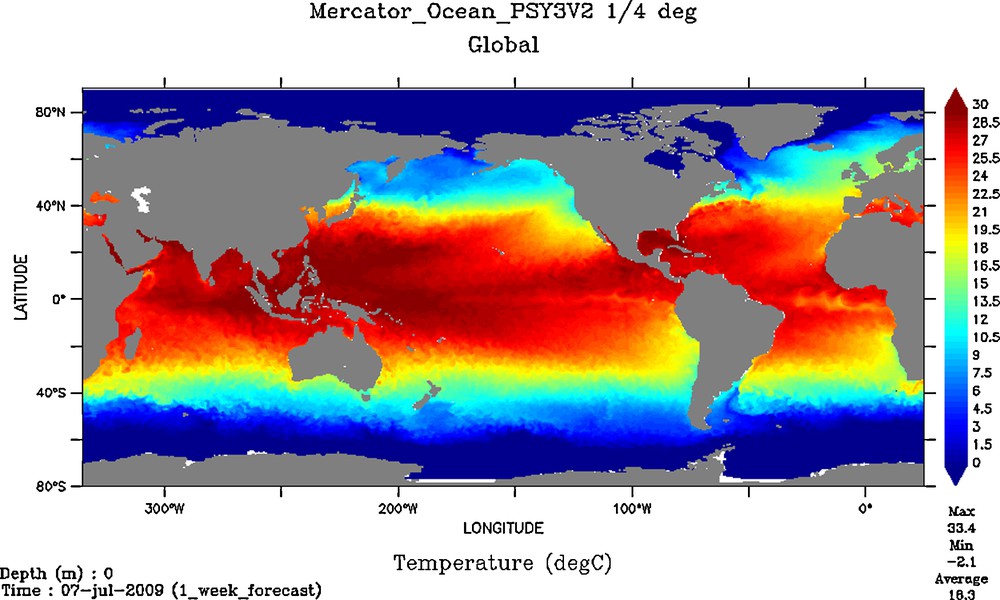
Surface temperature of the Atlantic ocean. The temperature ranges from 0° (blue colour) to 30° (red colour). According to Mercator Toulouse, France, 2009, http://www.mercator-ocean.fr/. Copyright© 2001–2009 Mercator Océan.
Température de surface de l’océan Atlantique. Les températures vont de 0° (couleur bleue) à 30° (couleur rouge). D’après Mercator Toulouse, France, 2009, http://www.mercator-ocean.fr/. Copyright© 2001–2009 Mercator Océan.
As is known, the El Niño/la Niña events are also very good examples of interactions between winds and oceans; the winds can displace hot water masses of the tropical Pacific Ocean towards Peru (El Niño) or Australia (La Niña) according to the regime and the strength of winds (Fig. 8a, b).
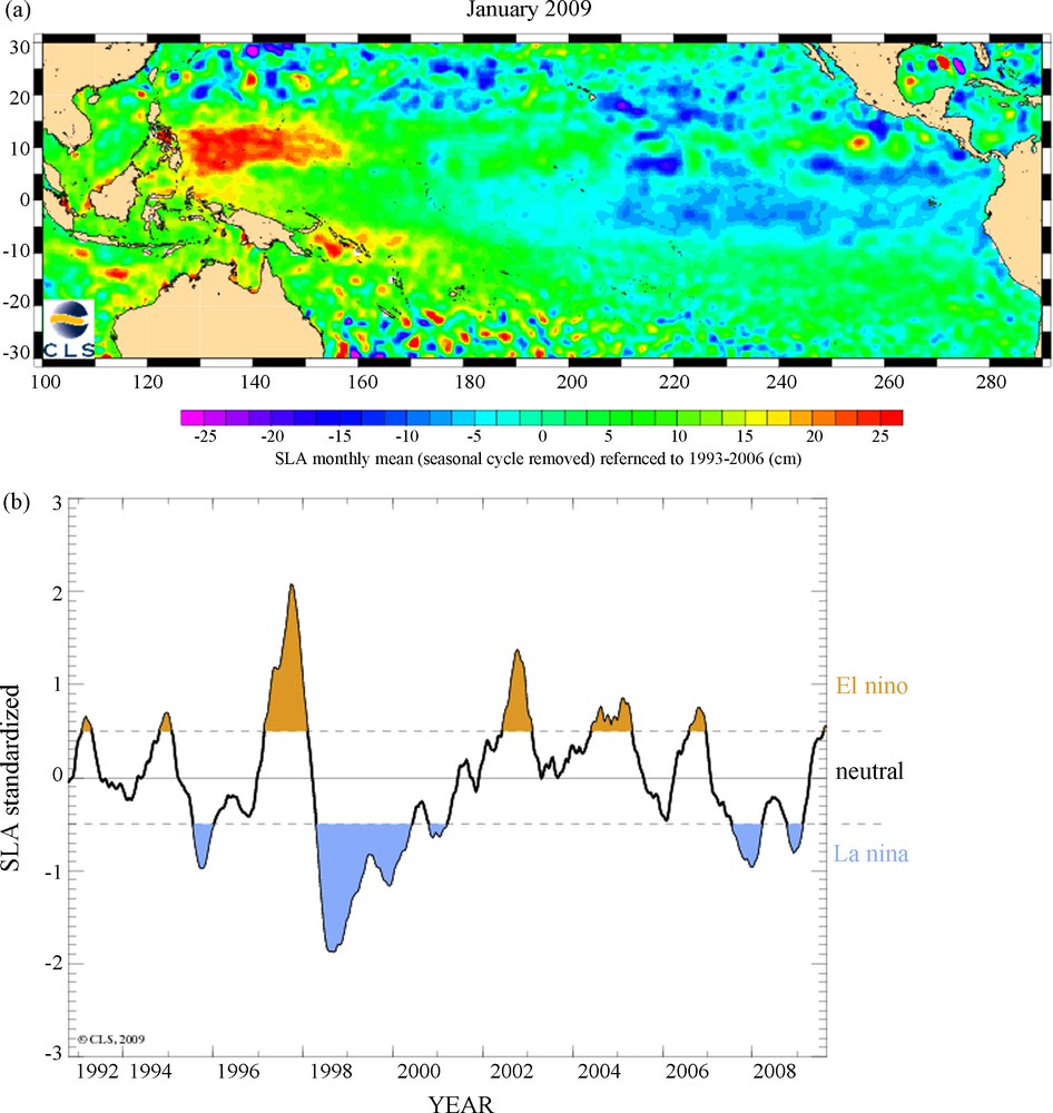
a: sea level anomaly in January 2009, referenced to the mean sea surface level for the 1993–2006 period. Violet colour corresponds to a lower level of 20 cm and red colour to a higher level of 25 cm. Seasonal cycle is removed. http://www.aviso.oceanobs.com/en/news/ocean-indicators/el-nino-bulletin/index.html. Copyright© 1997–2008, CNES/ CLS; b: mean sea level anomaly in the tropical Pacific as a function of years referenced to the mean sea level for the 1993–2006 period. Yellow colour corresponds to a higher level (El Niño), blue colour to a lower level (La Niña). http://www.aviso.oceanobs.com/en/news/ocean-indicators/el-nino-bulletin/index.html. Copyright© 1997–2008, CNES, CLS.
a : anomalies du niveau de la mer observées en janvier 2009 par rapport au niveau moyen défini sur la période 1993–2006. La couleur violette correspond à un niveau plus bas de 20 cm et la couleur rouge à un niveau plus haut de 25 cm. Le signal saisonnier a été supprimé. http://www.aviso.oceanobs.com/en/news/ocean-indicators/el-nino-bulletin/index.html. Copyright© 1997–2008, CNES/ CLS ; b : anomalie du niveau moyen de la mer dans le Pacifique tropical au cours de plusieurs années par rapport à une référence définie sur la période 1993–2006. La couleur jaune correspond à un niveau plus élévé (phénomène El Niño), la couleur bleue à un niveau plus bas (phénomène La Niña). http://www.aviso.oceanobs.com/en/news/ocean-indicators/el-nino-bulletin/index.html. Copyright© 1997–2008, CNES, CLS.
In the tropical Pacific Ocean in the area of 30° to −30°of latitude, sea level anomalies can be observed when comparing the mean monthly sea level to an average determined over the 1993–2006 period (Sea Level Anomalies [SLA] – Fig. 8a for January 2009). There are years when the mean sea level is higher than average (El Niño) and others when it is lower (La Niña) (Fig. 8b). In parallel as observed (http://bulletin.aviso.oceanobs.com/images/produits/indic/enso/time_curves/Msla_nino34_F6.png), the mean temperature of the ocean is higher during an El Niño event and lower in a La Niña event. The 1997–1998 El Niño event was quite exceptional; during the 2007–2008 period, the tropical Pacific was comparatively colder by few degrees Celsius. One cannot understand ocean currents by ignoring the winds. Thus, the combination of data issued of missions such as ADM-Aeolus (to be launched in 2010) or Jason-2 (launched in 2008) should provide a relevant information on the wind and the displacement of water masses.
3.3 Examples of interaction between biosphere, solid surface and atmosphere: Carbon cycle
The cycles of constituents such as H2O, CO2, CH4 are good illustrations of the interactions between the atmosphere and the lower layer and have to be taken into consideration. Fig. 9 (Trompette, 2003, pp. 282) illustrates the carbon cycle, which is of particular importance because it has its specific role in the greenhouse effect. On the Fig. 9, the emissions of carbon to the atmosphere are indicated from various origins (volcanic, anthropogenic, decomposition of rocks, weathering of rocks, respiration) and the possible mode of absorption (photosynthesis, dissolution in oceans, precipitation of carbonates). The CO2 concentration increases from about 310 in 1960 to about 385 parts per million by volume in 2009.
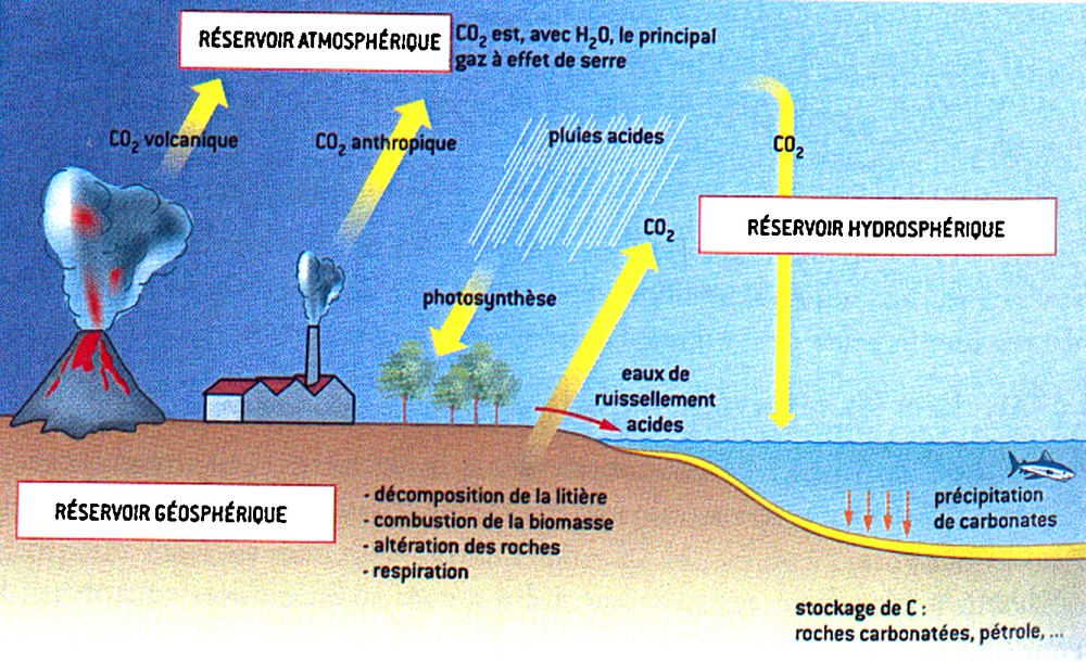
Simplified carbon cycle with the different reservoirs, in the atmosphere, hydrosphere, geosphere. The biosphere reservoir in itself includes living organisms at the surface of the geosphere and in the hydrosphere. According to Trompette, 2003, pp. 282.
Cycle du carbone simplifié avec les différents réservoirs atmosphérique, hydrosphérique, géosphérique. Le réservoir biosphérique en lui-même comprend des organismes vivant à la surface de la géosphère et dans l’hydrosphère. D’après Trompette, 2003, pp. 282.
Of course, a cycle such as the water cycle has also to be noted and it is also of particular importance with its geophysical and hydrological features: evaporation, storage in the form of ice, underground aquifers, fossil water, lakes and rivers, rain and drought, moisture in the atmosphere and in the soil, increase of mean sea level. All these features show the great importance of this cycle. It is the same for the nitrogen cycle.
Finally, what we learned from the observations of these cycles is also the ability of the Man with his societal behaviour to modify his environment. The nature of the soils that feed us, the water we drink, the air we breathe all the things that are vital to humanity have evolved over geological time, but we know that the Man can change them and this in time scales that have prevented the maintenance of a natural balance, a rhythm which does not allow Nature to react and to remain in a state of equilibrium and to slow towards a negative evolution for Man. The Earth is fragile and sometimes unstable with limited resources (Nahon, 2008). Man has many challenges to be tackled and won.
However, Man himself can react, at least to limit or slow down the degradation and pollution he has generated; this he begins to do. But at the same time, as it is very difficult to estimate the possible amplitude of this reaction, which creates large uncertainties in the scenarios that one should consider for the future. This explains, for example, the range of a possible mean temperature increase considered from 1.5 to 5 °C in the IPCC scenarios for the present century (IPCC stands for Intergovernmental Panel on Climate Change). Making predictions about the Earth's future is thus very difficult, but trying to do this as precisely as possible, continuously, with perennial and permanent observations of the Earth system, is certainly of primary importance.
In conclusion, all the layers of the Earth system are linked. Everything is interdependent, and it would be illusory to want to understand the Earth system and, in particular, the atmosphere, without taking into account all these interactions and interdependencies.
4 Conclusions
Many changes have taken place in the last 50 years in the study of the dense atmosphere (0–85 km). New high-performance technologies have been developed for in situ measurements or remote sensing observations. Initially, most of the information relevant to the upper atmosphere was gathered through the use of rockets. Satellites have then not only considerably extended the Earth observing capabilities but also literally changed the human vision of planet Earth. Nowadays, the observation of the Earth's atmosphere is still expanding and great hopes lie within new mission concepts, such as the ADM-Adeolus to be launched in 2010. In the mean time, aircraft and balloons continue to play a role in everyday life, especially for weather forecasting. Considerable progress has been made at the scale of 4 to 7 days, which is very important from a societal point of view and should be emphasized. Understanding the phenomena involves also taking into account the incoming radiation and particles from the Sun and the remote environment. The ocean-atmosphere interactions and the atmosphere-land interactions are also of great importance. As a result data gathering, data analysis, data assimilation and modelling are of a growing complexity and more and more difficult to manage.
Another point to stress concerning the dense atmosphere is the great importance of many societal aspects: climate change and environmental pollution, which have to be considered now in parallel with all scientific issues. Considering all these issues requires new governance processes to be addressed at the highest level of state, and at the European and international levels (GMES in Europe and GEO/GEOSS at the international level). To achieve these objectives, the continuity of observations is a fundamental point. Continuous observations are needed over time and it is also necessary that these observations and measurements be accurate and validated continuously.
One important point remains to be emphasized. All these tasks could not be developed without the immense progress made in the field of information exchange and in the formation of databases. It is mandatory to archive perennially the data after their validation and calibration. High-speed computer networks (Internet development) and the general advancement of information technology are also essential.
Acknowledgements
We are very much indebted to Pierre Baüer and the reviewer for very interesting remarks, discussions and pertinent advice.