

1 Introduction
Attempts to use seismic waves for the detection of material changes in the subsurface started about 30 years ago. During the last five year, however, the interest in this topic drastically increased because of the new observational possibilities provided by the noise based approach. We begin this article with an introduction of investigations made with impulsive sources and continue with an overview of recent noise based investigations. In the last part of the introduction we discuss causes of seismically detected changes mostly in the context of fault zones. The principles of passive image interferometry (PII) as the tool for noise based monitoring is introduced in Section 2. In Sections 3, 4, and 5 we present applications of passive image interferometry to three different environments. Section 3 discusses the investigation of PII to Merapi volcano where velocity changes are interpreted as being caused by hydrological effects. Possibilities of monitoring changes in fault zones with PII are discussed in Section 4 using examples from Japan. A rather exotic example of seismological monitoring is presented in Section 5 where we analyze changes in the lunar subsurface.
1.1 Change detection in seismology
It is well known that the Earth is not static, but dynamically evolves in time. At plate boundaries according to elastic rebound theory plates move and slowly deform. When their internal strength is exceeded, energy is suddenly released in an earthquake with fast ground deformation. Likewise volcanic processes such as inflation of magma chambers lead to deformations of the crust.
Deformations at the Earth’s surface related to plate motion, earthquakes, and volcanoes can be directly observed with GPS and InSAR techniques. Measuring the effects of such temporal variations inside the Earth using seismic imaging, turned out to be difficult.
The most reliable results are expected for repeated experiments, where the same seismic source and receiver positions are used several times resulting in identical seismic ray path. One common configuration is to use repeated explosive sources, which are recorded at identical seismometer positions (Li et al., 1998, 2003, 2006; McEvilly and Johnson, 1974; Nishimura et al., 2000; Vidale and Li, 2003). The disadvantage of such studies is that repeated explosions are expensive and, therefore, generally few repetitions are done resulting in a poor temporal sampling. The destruction of the source area is another problem of explosives and limits the reproducibility.
Shorter repeat times and a better reproducibility of the source signal can be obtained by other artificial sources such as airguns shot in water basins (Ando et al., 1980; Hashida et al., 1981; Leary et al., 1979; Reasenberg and Aki, 1974; Wegler et al., 2006) or vibrator sources (Clymer and McEvilly, 1981; De Fazio et al., 1973; Ikuta et al., 2002; Karageorgi et al., 1997; Yukutake et al., 1988). Generally, such sources are less powerful than explosions and can cover only smaller areas. 100 ton seismic vibrators, where the seismic signals can be recorded up to 300–400 km from the source (Kovalevsky, 2008), are exceptional and the logistical and financial effort for such experiments is high.
Poupinet et al. (1984) pointed out that it is also possible to use the coda of similar earthquakes (earthquake multiplets) to extract temporal variations in seismic velocity. In case of a homogeneous change in velocity the arrival time of coda waves shifts proportional to lapse time. Therefore, time shifts in the coda are generally larger than time shift of direct P- and S-waves. Since the earthquake sources are deep, the observed temporal variations of velocity are less influenced by the shallow subsurface layers. On the other hand, the occurrence of similar earthquakes is irregular and cannot be influenced, which often results in poor temporal coverage of the velocity changes.
Snieder et al. (2002) and Snieder (2006) clarified the theoretical background of the technique to use coda waves for the detection of material changes and termed it Coda Wave Interferometry. These authors showed that a small change in velocity results in a time shift and that it can be distinguished from a small change in scatterer distribution or a small change in source position, which both result in changes in the cross-correlation coefficient. Coda Wave Interferometry was applied to seismograms recorded on active volcanoes to monitor temporal variations of its structure (Pandolfi et al., 2006; Ratdomopurbo and Poupinet, 1995; Snieder and Hagerty, 2004; Wegler et al., 2006). Bokelmann and Harjes (2000) observed a decrease of 0.2% after hydraulic fracturing in Germany at the 9 km deep KTB borehole. Earthquake multiplets were also used to reveal a sudden decrease of seismic velocity followed by a gradual increase after the occurrence of large crustal earthquakes (Poupinet et al., 1984; Schaff and Beroza, 2004; Rubinstein and Beroza, 2004a,b, 2005; Li et al., 2006; Peng and Ben-Zion, 2006; Rubinstein et al., 2007).
1.2 The use of ambient noise for the detection of changes
Recently, besides artificial sources and natural earthquake sources ambient seismic noise was also suggested as a possible seismic source to monitor temporal variations using a technique called passive image interferometry (Wegler, 2006; Nakahara et al., 2007; Ohmi, 2007; Sens-Schönfelder and Wegler and Sens-Schönfelder, 2007; Brenguier et al., 2008a,c; Ohmi et al., 2008; Duputel et al., 2009; Wegler et al., 2009; Mordret et al., 2010). In this method as a first step, the elastic Green’s function between two seismometers is constructed using the cross-correlation of seismic noise recorded at the two sensors. For seismology, this noise correlation technique was first suggested by Shapiro and Campillo (2004) and Shapiro et al. (2005). Then in a second step, the Green’s functions obtained for different periods are treated as similar earthquakes and Coda Wave Interferometry is used to extract a temporal variation in seismic velocity. The first application was presented by Sens-Schönfelder and Wegler (2006), who revealed seasonal variations of seismic velocities at Merapi volcano, Indonesia, caused by precipitation. Wegler and Sens-Schönfelder (2007) and Wegler et al. (2009) observed a sudden decrease of seismic velocity after the 2004 Mid-Niigata earthquake, Japan. Nakahara et al. (2007), Ohmi (2007), Brenguier et al. (2008a), Ohmi et al. (2008), applying the same technique observed similar effects for the 2007 Noto Hanto, for the 2007 Niigata-Ken Chuetsu-Oki, for the 2005 Fukuoka-Ken Seiho-Oki, and for the 2004 Parkfield earthquakes, respectively. Brenguier et al. (2008c) and Duputel et al. (2009) used the method at Piton de la Fournaise volcano, La Réunion Island. These authors observed consistent decreases in seismic velocity a few weeks before eruptions and proposed the technique as a possible forecasting tool. Mordret et al. (2010) applied PII to Mt. Ruapehu, New Zealand. These authors observed a decrease in seismic velocity of 0.8% 2 days before the 2006 eruption.
The advantages of using noise as a source are manifold. Since one of the receivers acts as a virtual source, the source region is not damaged as it is the case in explosion experiments or moved as it is the case for similar earthquakes. Moreover, in principle we may install both receivers in boreholes below the watertable and the weathering layer, which may solve the problem of near surface effects. Noise as a source is continuously available, which results in a dense temporal coverage of measurements. Using high frequency noise above 1 Hz Sens-Schönfelder and Wegler (2006) and Wegler and Sens-Schönfelder (2007) could construct Green’s functions for each day, whereas Brenguier et al. (2008c) and Wegler et al. (2009) using microseismic noise around 5 s averaged the Green’s functions of 10 days and 30 days, respectively. Finally, the method is easy to implement for existing permanent seismometers without expensive experiments.
1.3 Causes of seismically detected changes
In previous studies on temporal variations of seismic velocities, both, variations of tectonic origin and of non-tectonic origin have been observed. Typical non-tectonic effects influencing the seismic velocity in the shallow subsurface are rain, atmospheric pressure, and Earth tides. Clymer and McEvilly (1981) reported on seasonal oscillations of seismic velocities of 1%, which could be explained by rainfall induced variations in the degree of water saturation of the near-surface. Karageorgi et al. (1997) and Ikuta et al. (2002) also measured local near-surface effects on seismic velocity correlating with seasonal rainfall. A similar seasonal oscillation with variations of 2% was also observed by Sens-Schönfelder and Wegler (2006) for the Merapi volcano and the Los Angeles basin (Meier et al., 2010). De Fazio et al. (1973) and Reasenberg and Aki (1974) revealed a tidal effect on crustal seismic velocity. These authors observed a periodic semidiurnal oscillation with a peak-to-peak variation of relative velocity of 0.1% and 0.5%, respectively. This observation was confirmed by Bungum et al. (1977), Ando et al. (1980), and Yukutake et al. (1988), who measured peak-to-peak variations of 1.0%, 0.5%, and 0.1%, respectively. Such measurements were used to calibrate the stress sensitivity of velocity variations in shallow crustal rocks. Hashida et al. (1981), on the contrary, pointed out that such variations seem to be more efficiently induced by atmospheric pressure than by Earth tide strain.
A 0.2% velocity decrease related to the occurrence of the M 5.9 Coyote Lake, California, earthquake was observed by Poupinet et al. (1984) using an earthquake doublet consisting of two microearthquakes, that occurred 14 months before and 7 months after the main earthquake, respectively. The observation was interpreted as a decrease in static stress. Li et al. (1998) observed a velocity increase of 0.5–1.5% after the 1992 Landers earthquake. These authors used data from two explosion experiments two and four years after the 1992 Landers earthquake. The observation was interpreted as the closure of dry cracks as the crust heals after the earthquake. Nishimura et al. (2000) observed a 0.3–1.0% decrease of seismic velocity associated with the M 6.1, 1998 Iwate earthquake. These authors used two explosions that were carried out about one month before and two months after the main earthquake. Again a drop of static stress in the Earth crust was suggested as a mechanism. Vidale and Li (2003) continued the experiment of Li et al. (1998). One artificial explosion experiment every year or every two years near the source region of the Lander earthquake was carried out. The nearby Hector Mine earthquake caused a decrease of velocity. Afterwards, the velocity increased again. As possible interpretation of their observations the authors discuss a near surface damage due to strong shaking followed by healing, static stress changes, and changes in the degree of fluid saturation of fluid-filled cracks. Two explosions after the 1999 M 7.1 Hector Mine earthquake, each repeated once, were carried out by Li et al. (2003). The observed velocity increase was interpreted as a closure of cracks that opened in the Hector Mine earthquake. Using a vibrator source Ikuta et al. (2002) observed a delay in the S-wave arrival time due to the Western Tottori earthquake (M 6.6) in a distance of 180 km. Schaff and Beroza (2004) and Rubinstein and Beroza (2004a) analysed the 1989 Loma Prieta and the 1984 Morgan Hill, California, earthquakes. These authors pointed out that repeating aftershocks follow Omori’s law and, therefore, many repeating quakes are available when changes in seismic velocity are expected to be the largest. They observed coseismic decreases of velocity (1.5% for P and 3.5% for S) followed by a postseismic increase. The observation was interpreted as a nonlinear response to the main shock strong ground motion. Similar effects were also observed for the largest aftershock (Ml 5.4) of the Loma Prieta earthquake (Rubinstein and Beroza, 2004b). Velocity variations caused by the 2004 Parkfield earthquake (M 6) were observed with surface and borehole stations in 70–350 m depth (Rubinstein and Beroza, 2005). These authors found less velocity reduction for borehole stations and concluded that changes mainly occur in the upper 100 m of the Earth. The same earthquake was also analysed by Li et al. (2006). These authors deployed a dense array of 45 seismometers. Additionally to repeated aftershocks they also analysed shot data from two shots in 2002 and in 2004 (3 months after the main shock), respectively. Again a co-seismic decrease of velocity followed by gradual healing was observed. Peng and Ben-Zion (2006) deployed a seismic network on the North Anatolian fault after the 1999 Mw 7.4 Izmit earthquake. Using aftershock multiplets of that earthquake and of the Mw 7.1 Düzce earthquakes, that occurred shortly after, they were able to resolve a sharp velocity reduction immediately after the Düzce earthquake followed by a gradual logarithmic-type increase. Rubinstein et al. (2007) observed a velocity decrease after the Tokachi-Oki earthquake. These authors also interpret their observations as a shallow effect near the receiver. Due to nonlinear strong ground motion near-surface material is damaged. Additionally, they state that within the rupture zone stronger reductions occur, which might be caused by deeper effects. Sawazaki et al. (2009) reported a drastic decrease of near surface velocity with the occurrence of the Western-Tottori earthquake using coda deconvolution of surface and 100 m deep borehole recordings.
Using passive image interferometry a temporal resolution as high as one measurement per day can be obtained. So far this technique was applied to the 2004 Mid-Niigata earthquake, Japan, (Wegler and Sens-Schönfelder, 2007; Wegler et al., 2009), to the 2007 Noto Hanto and the 2007 Niigata-Ken Chuetsu-Oki earthquake, Japan, (Ohmi, 2007; Ohmi et al., 2008), to the 2005 Fukuoka-Ken Seiho-Oki earthquake, Japan (Nakahara et al., 2007), and the 2004 Parkfield earthquake, California (Brenguier et al., 2008a). In all cases, a sudden decrease of seismic velocity at the time of the main shock could be revealed.
Although the fact of crustal seismic velocity reduction during a large crustal earthquake is now well established, the physical mechanism of its cause is still under debate. A recent overview of possible models is given by Rubinstein and Beroza (2004a) and Wegler et al. (2009). These authors discuss four different mechanisms, which may lead to a crustal velocity decrease. A static stress change causes a closure or opening of cracks, which may result in changes of velocity. Such changes will be deep and positive and negative velocity changes are expected corresponding to regions of increased and decreased stress. Secondly, pore pressure variations may cause changes in the hydrologic system. If the fraction of water in partially filled cracks changes, it can also influence the seismic velocity. The third model assumes a physical damage of the fault zone caused by the fault motion, which results in reduced velocity. Finally, a physical damage caused by non-linearity of strong ground motion can cause velocity decreases. Such changes are expected to be shallow and to correlate with the strength of shaking.
2 Passive image interferometry
The idea of passive image interferometry to monitor seismic velocity variations with ambient seismic noise was introduced by Sens-Schönfelder and Wegler (2006). The first of the two steps of PII is the construction of impulse responses between station pairs from continuous noise records. This process, known as passive imaging or seismic interferomery is well established in theory and practice (e.g. Gouédard et al., 2008; Wapenaar et al., 2010) and is the basis also for ambient noise tomography (Sabra et al., 2005; Shapiro et al., 2005). For the precision of PII it is important that the coda part of the Green’s function is contained in the noise cross-correlation function (NCF) and not only ballistic waves that are sufficient for tomography. This was demonstrated by Sens-Schönfelder and Wegler (2006) by showing the stability of the NCFs for lapse times much larger than the travel time of ballistic waves. Figure 2 shows NCFs obtained from the data of the Merapi seismic network (Fig. 1) that was operated by the Universität Potsdam and the GFZ-Potsdam (Wassermann, 2001). The two graphs compare NCFs for different station distances and frequency ranges. Time axis spans from August 1997 until June 1999 in both cases but the lapse time is ±50 s in A and ±8 s in B reflecting the different attenuation in the different frequency ranges. Despite the different distances and frequencies the NCFs show coherent phases at lapse times much larger than the ballistic travel time. Since the noise that is used to reconstruct the NCFs at different times is different, the coherent phases in the coda reflect properties of the propagation medium. This finding allows one to obtain information about the medium form coda part of the NCFs which is particularly sensitive to weak material changes.
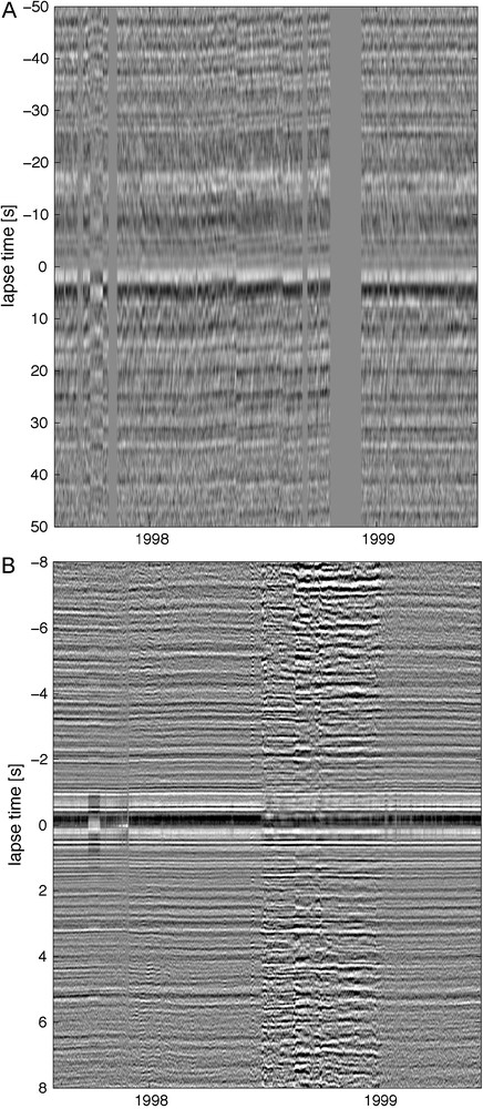
Temporal stability of the NCFs within the Merapi network. A: Daily NCFs for the sensors A1 and C1 (arrays KEN and GRW) in the frequency band 0.1–1 Hz; B: Daily NCFs for the sensors C1 and C2 (within array GRW) in the frequency band 0.5–24 Hz (from Sens-Schönfelder, 2008).
Stabilité temporelle de NCF (fonctions de corrélation de bruit) dans le réseau du Merapi: A: NCFs journaliers pour les capteurs A1 et C1 (réseaux KEN et GRW) dans la bande de fréquence 0,1–1 Hz; B: NCFs journaliers pour les capteurs C1 et C2 (à l’intérieur du réseau GRW) dans les bande de fréquence 0,5–24 Hz (selon Sens-Schönfelder, 2008).
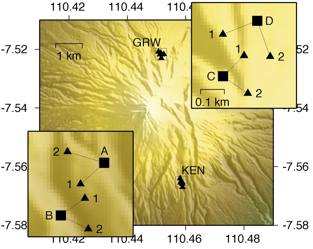
Location of seismic stations on Mt. Merapi (from Sens-Schönfelder, 2008).
Localisation des stations sismiques sur le Mt Merapi (selon Sens-Schönfelder, 2008).
Although the phases such as individual maxima can be traced over the whole study period in both graphs of Fig. 2 there is notable variation in their lapse time. The quantification and interpretation of these variations is the second step of PII. It is analogous to coda wave interferometry for directly recorded impulse responses (Snieder, 2006). There are different types of changes that may occur in the investigated media with different manifestations in the signals. A simple possibility is that the medium gets distorted such that scatters change their effective scattering cross section. This may happen when magma is emplaced in empty parts of a volcano’s plumbing system or when the structure of the medium changes for example in the collapse of a volcanic dome or along the rupture of an earthquake. Such changes would result in a decorrelation of the waveforms that would generally increase with increasing lapse time.
A change in the propagation velocity would in contrast result in travel time changes of the seismic phases. Since in the case of a homogeneous velocity variation this travel time change δτ is proportional the lapse time τ of the phase, the wave forms will simply be stretched or compressed as result of the velocity change. This is the case in Fig. 2B where the phases (e.g. around 5 s lapse time) show significant travel time variations. The fact that the variations for positive and negative lapse times are symmetric about zero lapse time is a signature of the stretching of the wave form caused by changing subsurface velocity. In contrast the lapse time changes in Fig. 2A are anti-symmetric. Such a behavior is the result of badly synchronized seismometer clocks (Stehly et al., 2007). The observation of such changes in the NCFs can be used to estimate the clock errors directly from the seismic data in order to synchronize data from a seismic network after the recording (Sens-Schönfelder, 2008).
No matter which effect is dominant, the change of the NCFs has to be quantified in comparison to some reference. For weak changes encountered in seismology a long term stack of the NCFs proved to provide good reference traces.
When wave form changes are evaluated it is mostly assumed that the causative alteration of the medium is a spatially homogenous change of the seismic velocity. This is a first order approximation only, but without independent knowledge about the type and distribution of the medium variation, the assumption is reasonable. Since the change of the NCFs that is expected for this assumption is a waveform stretching it is most natural to simulate this stretching when the change is quantified. This was first suggested and used by Sens-Schönfelder and Wegler (2006). The stretching technique thus compares the reference trace hr(τ) with stretched and compressed version of the current NCF hc(τ, t) obtained from noise recorded in some time interval of length T centered around time t. In practice, the stretching is done by resampling the NCF with a sampling rate increased by a factor 1 − ɛ. The similarity between the reference and current NCFs is evaluated by means of the correlation coefficient R(ɛ, t) of the two NCFs for a given stretching ɛ in some lapse time window [τmin, τmax]:
| (1) |
| (2) |
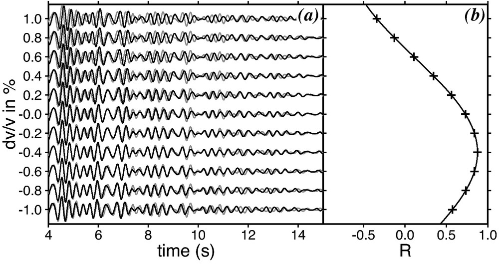
Example for the estimation of the velocity change with the stretching technique. (a): Eleven identical reference traces (long term average of NCF) in the lapse time window from 4 to 15 s for the autocorrelation at the japanese station KZK in the frequency band 2 – 8 Hz in gray. Overlain in black are 11 stretched/compressed autocorrelation functions generated from noise that was recorded October 1 2004. The assumed relative change in velocity
Example for the estimation of the velocity change with the stretching technique. (a): Eleven identical reference traces (long term average of NCF) in the lapse time window from 4 to 15 s for the autocorrelation at the japanese station KZK in ... Lire la suite
Exemple d’estimation de la modification de la vitesse par technique d’étirement (stretching) (a) Onze traces de référence identiques (moyenne long terme de NSF) dans la fenêtre d’intervalle de temps de 4 à 15 s pour l’auto-corrélation, à la station japonaise KZK dans la bande de fréquence 2–8 Hz en grisé. Surlignées en noir, onze fonctions d’auto-corrélation après compression/étirement, générées par le bruit enregistré le 1er Octobre 2004. Le changement relatif de vitesse
Exemple d’estimation de la modification de la vitesse par technique d’étirement (stretching) (a) Onze traces de référence identiques (moyenne long terme de NSF) dans la fenêtre d’intervalle de temps de 4 à 15 s pour l’auto-corrélation, à la station japonaise KZK ... Lire la suite
Another possibility to estimate the velocity change is to measure the time shifts dτ in various short lapse time windows. Plotting δτ as a function of τ and the slope will provide δτ/τ. This approach was suggested by Poupinet et al. (1984). It was termed Moving-Window Cross Spectral analysis by Ratdomopurbo and Poupinet (1995) because it estimates the time shifts δτ from phase shift in the cross-spectrum. Snieder et al. (2002) suggested to measure the time shifts directly in the time domain. The advantage of the stretching technique over the linear fitting of the δτ(τ) function was pointed out by Hadziioannou et al. (2009). The stretching technique is far less sensitive to noise so that reliable measurements can be obtained even if signal and noise are of the same amplitude. Today most investigations apply the stretching technique from Sens-Schönfelder and Wegler (2006) to estimate the velocity change.
No matter which technique is used to obtain ɛm, the procedure is repeated for current NCFs from all possible times t during the study period. This provides a time series ɛm(t) that measures the time evolution of the subsurface velocity changes. A measure that quantifies how well the wave field alteration can be modeled by the spatially homogeneous velocity variation is the time series R(ɛm(t), t) (Eq. (1)). It measures the similarity of the reference and the current NCF after the effect of the velocity change has been corrected for by stretching the wave form. The time series ɛm(t) and R(ɛm(t), t) quantify the response of the wave field to an alteration of the subsurface. They are the main result of an analysis with passive image interferometry.
In the next sections we review various application of PII to different environment and discuss interpretations of the identified subsurface changes.
3 Velocity variations induced by ground water level changes at the Merapi volcano, Indonesia
The idea to monitor subsurface velocity variations with seismic noise correlations was presented by Sens-Schönfelder and Wegler (2006) in an application to data from the Merapi volcano.
Since 1997 three seismic arrays have been operated on Mt. Merapi (Wassermann, 2001). We focus on data from stations GRW0 and GRW1 (sensors C1 and C2 in Fig. 1) because these sensors were connected to a common digitizer which provides precise relative timing avoiding shifts of the NCFs as observed in Fig. 2A. Data are almost continuous between August 1997 and June 1999.
NCFs are retrieved by cross-correlating different one-day seismic records that are highpass-filtered at 0.5 Hz. To down-weight the contribution of coherent phases such as teleseismic body waves in the correlations we clip the records at one standard deviation of the recorded seismic noise. The resulting NCFs are shown in Fig. 2B. Before the application of the stretching technique we averaged the causal and acausal parts of the cross-correlation functions.
We estimate velocity changes for each one-day NCF (between station GRW0 and GRW1) with respect to a reference trace assuming that
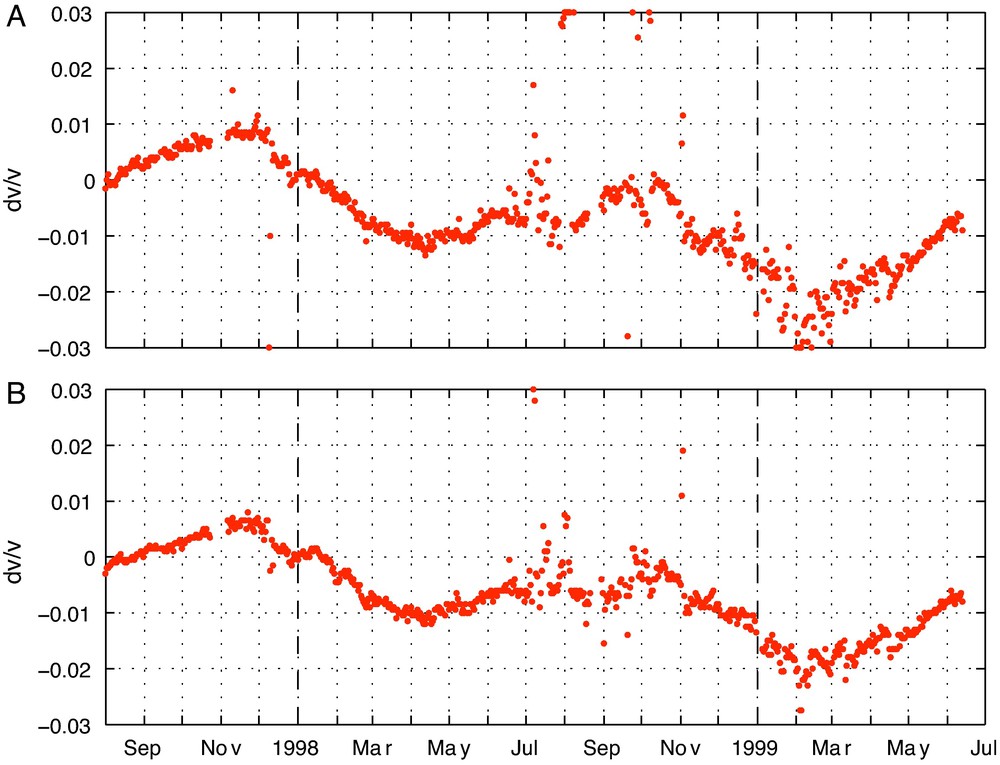
Velocity variations at Mt. Merapi obtained from the TT component of the GT between the stations GRW0 and GRW1 (A) and obtained from the auto-correlation of the east component of station GRW1 (B) (from Sens-Schönfelder and Wegler, 2006).
Modifications de la vitesse au Mont Merapi, obtenues à partir de la composante TT du tenseur de Green entre les stations GRW0 et GRW1 (A) et à partir de l’auto-corrélation de la composante est de la station GRW1 (B) (selon Sens-Schönfelder and Wegler, 2006).
The blue and green curves in Fig. 4A show results of CWI measurements (Wegler et al., 2006) made at the GRW and KEN arrays with active sources. Considering the daily variability of our measurements and the source receiver distance of more than 3 km used for the active measurement, we conclude that our measurements are in agreement with the results of the active experiment.
The periodicity of the velocity fluctuations of approximately one year in this tropical environment suggests a climatic influence most likely by precipitation. Another observation also supports a connection with precipitation: The amplitude of the estimated velocity variations depends on the lapse time at which they are measured in the NCFs. This has never been reported for CWI measurements before and indicates that the velocity perturbations are spatially inhomogeneous. We can explain this observation together with details of the temporal variation with a hydrological model of the ground water level (GWL).
The model is illustrated in Fig. 6. We assume that drainage of ground water occurs through a stationary aquifer that can approximately be described by Darcy’s law. Then the drainage is proportional to the height of the ground water table which results in an exponential decrease of the water level after rain events. A convolution of the precipitation rates with this exponential function thus gives the GWL (below surface) at time ti:
| (3) |
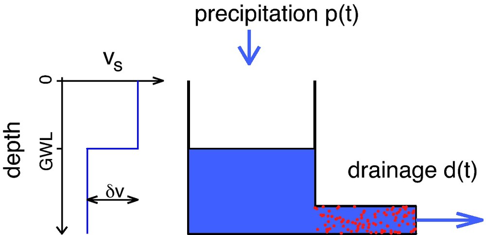
Illustration of the hydrological model for the velocity changes observed at Mt. Merapi. Right hand side shows the hydrological system that is charged by precipitation and discharged through a Darcy-like aquifer. Left hand side shows the resulting velocity. Changes in the hight of the ground water level (GWL) will move the velocity discontinuity.
Schéma du modèle hydrologique pour les modifications de vitesse observées au Mont Merapi. A droite, le système hydrologique chargé par les précipitations et déchargé par l’intermédiaire d’un aquifère de type Darcy. A gauche, la vitesse résultante. Les modifications dans la hauteur du niveau de l’eau souterraine (GWL) déplacent la discontinuité de la vitesse.
To relate the ground water level with delay times we define the depth (z) and time dependent relative velocity perturbation V(ti, z) and a reference water level GWLref that we choose equal to the mean level of January 1998. Then
| (4) |
| (5) |
The diffusivity constant D = 0.05 km/s2 as estimated at Mt. Merapi by Wegler and Lühr (2001) is used. The kernel K(z, τ) is illustrated in Fig. 7 for lapse times τ = 3 s and τ = 7 s.
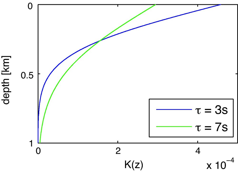
Sensitivity kernel of PII measurements for velocity changes at different depths.
Noyau de sensibilité des mesures de PII pour les modifications de vitesse à différentes profondeurs.
The result of the hydrological modeling is shown in Fig. 4B. It shows the daily rainfall as input data, the inferred GWL and the modelled apparent homogeneous velocity variation for the 2–4 s and 6–8 s time windows that may be compared with the measured values. Considering that the precipitation data are averages over an area of approximately 100 by 100 km and the simplicity of our hydrological model we can explain the velocity variations in remarkable detail. The model also explains the difference between the blue and the red curves in Fig. 4B that represent the measurements at different lapse times. We are thus confident that the observed velocity variations are related to precipitation via changes in the ground water level. The successful explanation of the lapse time dependence of the relative delay times by depth dependent velocity perturbations indicates that the high frequency coda is made up of scattered body waves rather than surface waves.
The benefit of this investigation is the comparison of the two completely different data sets. With the hydrological model that relates precipitation data with seismic noise record we provide an independent check for PII.
4 Co-seismic changes of seismic velocity in Japanese fault zones
PII is suitable for resolving small (≈ 0.1%) co-seismic velocity changes in the source region of large, crustal earthquakes (Brenguier et al., 2008b; Ohmi et al., 2008; Wegler and Sens-Schönfelder, 2007; Wegler et al., 2009). One of the best studied examples is the 2004 Mw 6.6 Mid-Niigata earthquake, where ambient seismic noise recorded at Japanese Hi-net and F-net was used. Different frequency bands of noise can be used to construct NCFs. Using high frequency noise (e.g. 2–8 Hz) one day of data is generally sufficient to estimate the source-receiver co-located Green’s function. As the first step of PII, Fig. 8 shows an example of high frequency NCFs at a seismometer located 24 km from the hypocentre. A systematic time-shift between the NCFs before and the NCFs after the Mid-Niigata earthquake can be observed optically. In the second step of PII, the quantitative inversion for velocity changes, the NCFs for each day are treated as similar earthquakes or repeated shots. Using the stretching technique, a sudden drop in seismic velocity on the day of the earthquake can be inferred (Fig. 9).
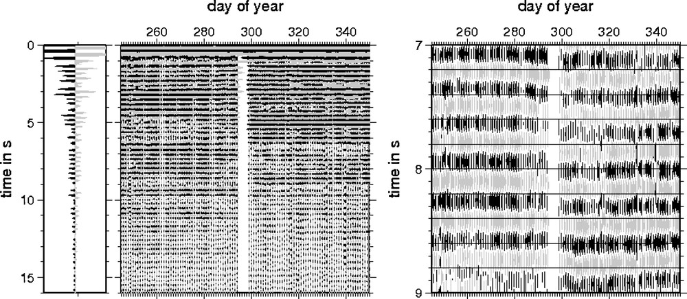
Auto-Correlation function of ambient seismic noise recorded during a period of 100 days at a distance of 24 km from the hypocentre of the Mid-Niigata earthquake. The auto-correlation function is computed from one day of noise and shown as a function of the day of the year. The black arrows indicate the day of the Mid-Niigata earthquake. Very left: NCF averaged over 100 days. Left: Large time window (0–15 s). Right: Small time window (7–9 s) (modified from Wegler and Sens-Schönfelder, 2007). Masquer
Auto-Correlation function of ambient seismic noise recorded during a period of 100 days at a distance of 24 km from the hypocentre of the Mid-Niigata earthquake. The auto-correlation function is computed from one day of noise and shown as a ... Lire la suite
Fonction d’auto-corrélation du bruit sismique ambiant, enregistré pendant une période de 100 jours, à une distance de 24 km de l’hypocentre du tremblement de terre de Mid-Niigata. La fonction d’auto-corrélation est calculée à partir d’un jour de bruit et présentée en fonction du jour de l’année. Les flèches noires indiquent le jour du tremblement de terre de Mid-Niigata. Tout à fait à gauche: NCF moyennée sur 100 jours. A gauche: Fenêtre de temps large (0–15 s). A droite: Fenêtre de temps étroite (7–9 s) (modifié d’après Wegler and Sens-Schönfelder, 2007). Masquer
Fonction d’auto-corrélation du bruit sismique ambiant, enregistré pendant une période de 100 jours, à une distance de 24 km de l’hypocentre du tremblement de terre de Mid-Niigata. La fonction d’auto-corrélation est calculée à partir d’un jour de bruit et présentée ... Lire la suite
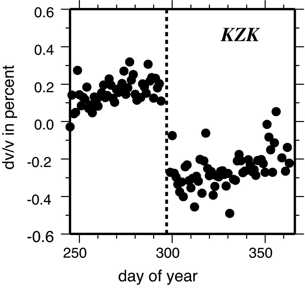
Relative change in seismic velocity
Changement relatif de vitesse sismique
PII can be applied to different station combinations, different frequency bands and different components of the Green’s tensor. Using lower frequencies (e.g. 0.1–0.5 Hz) longer noise time series of the order of weeks are required to construct stable Green’s functions. The advantage of using lower frequencies is that Green’s functions for larger station distances can be computed. Since the coda waves that are mainly used in PII are recorded on all three components of the seismometer, all 9 components of the Green’s tensor can be used to infer velocity changes.
Finally, the observed velocity changes have to be interpreted. All results using different station combinations, different components of the Green’s tensor, and different frequency bands are summerized in Fig. 10. In Mid-Niigata either a constant velocity or a drop in velocity for all combinations of station pairs is observed, whereas an increase of velocity is not observed. This is consistent with results at other fault zones (e.g. Brenguier et al., 2008b; Nishimura et al., 2000; Poupinet et al., 1984). Generally, it is difficult to invert for the exact location of the velocity change, because the theory in Eq. (2) is based on a spatially homogeneous change. Figure 10 shows that the area of decreased velocity roughly correlates with the source area of the earthquake. The physical mechanism causing co-seismic velocity drops during large crustal earthquakes is still under discussion. A nonlinear site response in the shallow subsurface layer can explain why velocity drops. However, the fact that the velocity decrease measured in the 2–8 Hz frequency band has a similar amplitude to the velocity decrease measured in the 0.1–0.5 Hz frequency band is an indication that the change is not restricted to the shallow subsurface. Static stress changes and coseismic water-level changes, in contrast, cannot explain the fact that only decreases in velocity are observed. For these models one would also expect certain areas of co-seismic increase of velocity, which have not been observed so far. The creation of a damage area within the fault zone is consistent with the data, but also a combination of several causes is possible.
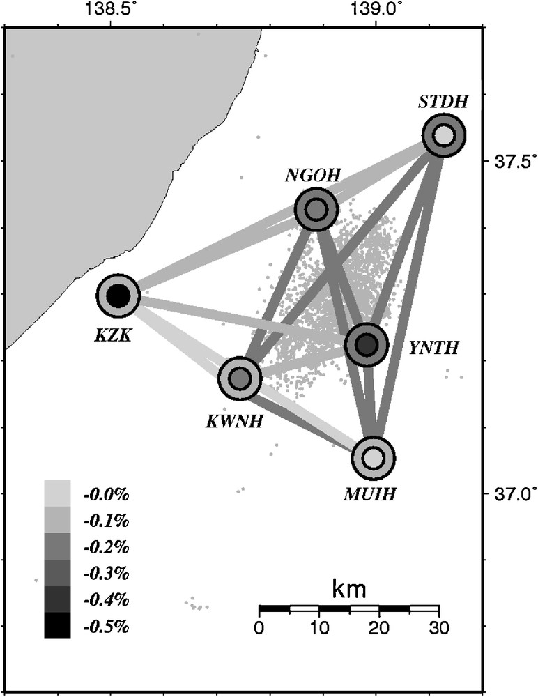
Observed decreases of seismic velocity in Mid-Niigata. Lines connecting two stations correspond to measurements using a NCF at these two stations (band pass filter 0.1–0.5 Hz). Large circles correspond to measurements using an auto-correlation of noise and a band pass filter of 0.1–0.5 Hz, whereas small circles indicate the results using a band pass filter of 2–8 Hz. Black indicates the largest decreases of –0.5% and light grey indicates no decrease (modified from Wegler et al., 2009).
Décroissance observée de la vitesse sismique à Mid-Niigata, les lignes reliant deux stations correspondant aux mesures utilisant une NCF entre ces deux stations (filtre à bande passante de 0,1–0,5 Hz). Les grands cercles correspondent aux mesures utilisant une auto-corrélation de bruit et un filtre à bande passante de 0,1–0,5 Hz, tandis que les petits cercles indiquent les résultats utilisant un filtre à bande passante de 2–8 Hz. La couleur noire indique les plus grandes décroissances de –0,5 % et le grisé indique qu’il n’y a aucune décroissance (modifié d’après Wegler et al., 2009). Masquer
Décroissance observée de la vitesse sismique à Mid-Niigata, les lignes reliant deux stations correspondant aux mesures utilisant une NCF entre ces deux stations (filtre à bande passante de 0,1–0,5 Hz). Les grands cercles correspondent aux mesures utilisant une auto-corrélation de bruit ... Lire la suite
5 Temperature related velocity variations in the lunar subsurface
Fascinating observations of weak velocity variations have been made on Earth with PII (Sections 3 and 4). However, the Earth environment is very complex and observations may have various causes ranging from meteorology to tectonics.
The situation on the moon appears to be much better under control: the solar heating and tidal stresses which are the most probable sources of changes can be independently evaluated in a quantitative way. The purpose of this investigation is to determine the changes in the lunar crust and to show that they are generated by the solar heating. This allows to check the validity of the PII technique in a natural environment where the source of change is precisely known.
The properties of the seismic wave field on the moon are perfectly suited for the application of mesoscopic concepts. Pioneering works in the 1970’s have demonstrated the diffusive nature of seismic waves in the heterogeneous and highly fractured regolith. We can deduce from the envelopes of seismic records acquired with controlled sources that the shallow subsurface is highly scattering but weakly attenuating. This is characterized by a transport mean free path of the order of ℓ⋆ ≈ 100 m and an attenuation length of ℓa ≈ 5 km (Dainty and Toksöz, 1981). With a wavelength of the order of ten meters we work well in the mesoscopic regime.
As part of the Lunar Seismic Profiling Experiment the Apollo 17 crew installed 4 geophones at the Taurus-Littrow landing site on the moon. The configuration of the triangular array installation is shown in the inset of Fig. 11. From August 1976 until April 1977 the four geophones were continuously operated. In the present study we analyze this continuous dataset. As noted by Latham et al. (1973) and Larose et al. (2005) the ambient vibrations that are recorded on the moon are related to thermal moonquakes of which most are too small to be clearly detected. To verify this, the upper panel of Fig. 12 shows the noise level at the central station of the array. The noise amplitude peaks shortly before sunset and has a second peak right after sunrise. This is the expected behavior for energy released from thermally stressed rocks that is related to temporal changes of temperature. However, there is some indication that the local maximum of the noise amplitude in the morning of the lunar day might be related to inductive coupling of magnetic field changes into the coils of the geophones when the moon enters the Earth’s magneto tail (Sens-Schönfelder and Larose, 2010).
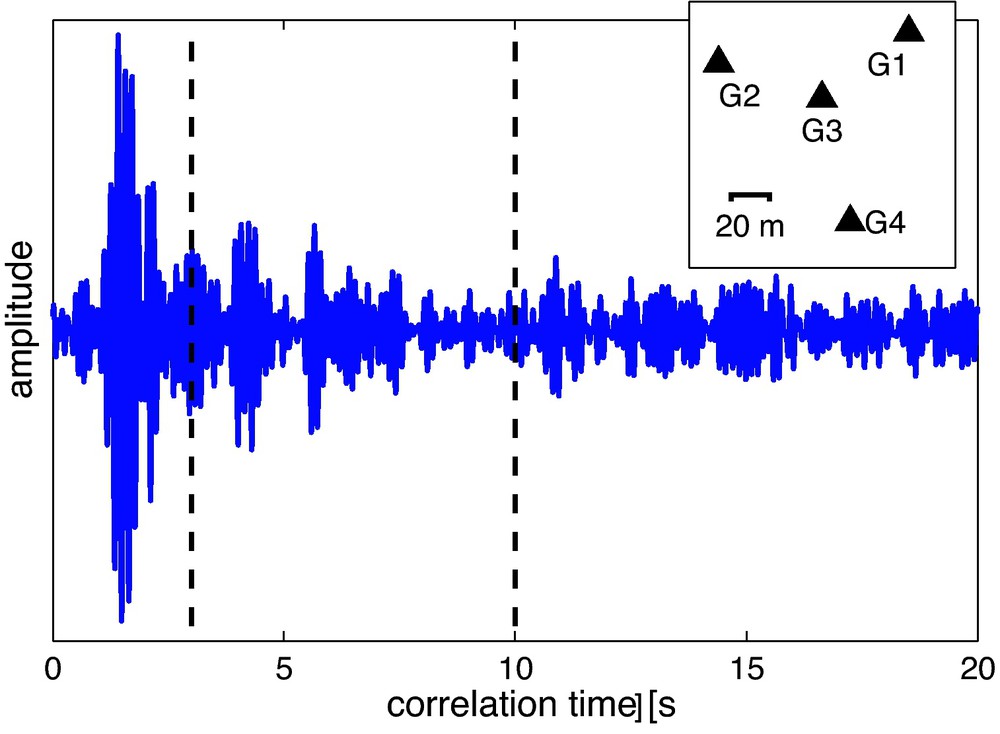
NCF between geophones G2 and G3 retrieved from ten days of noise around sunset. Insert: map of the geophone array (from Sens-Schönfelder and Larose, 2008).
NCF entre les géophones G2 et G3, récupérés à partir de 10 jours de bruit au coucher du soleil. En encart: la carte du réseau de géophones (selon Sens-Schönfelder and Larose, 2008).
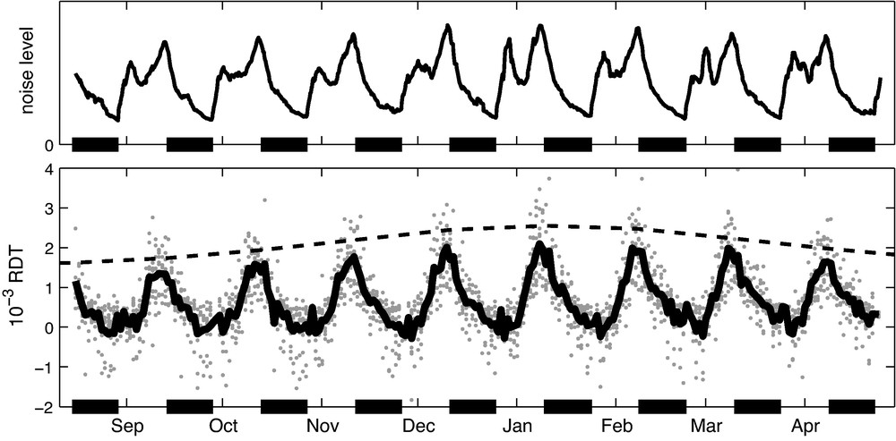
Noise level and relative delay time (RDT) variations of seismic waves in the shallow lunar crust. Upper panel: Variations of the noise level at the central station G3. Lower panel: Gray dots: individual measurements of the RDT. Continuous curve: average over the ten available station configurations. Dashed curve: qualitative course of the inflow of thermal energy at lunar noon. Bold line segments at the bottom of each panel indicate lunar night (from Sens-Schönfelder and Larose, 2008).
Energie du bruit et variation relative des temps de trajets des ondes sismiques dans la partie superficielle de la croûte lunaire. En haut: variations du niveau de bruit au capteur central G3. En bas, pointillés gris: mesure des variations relatives de délais; en ligne discontinue: variation qualitative du flux solaire au zénith lunaire. Les segments en gras au pied de chaque figure indiquent les périodes de nuit lunaire (selon Sens-Schönfelder and Larose, 2008).
The thermally generated seismic noise allows to retrieve approximations of Green’s functions between seismic sensors. With the four geophones it is possible to retrieve approximations of ten noise correlation functions (NCF), including auto-correlations. These NCFs are computed for the eight months of available data in segments of 24 hours. The records with a dynamic range of 7 bits are clipped at an amplitude of ±20 counts around the zero position. As an example of the correlation, we plot on Fig. 11 the NCF between geophones G2 and G3: a direct (Rayleigh) wave is reconstructed, followed by late arrivals scattered at surrounding heterogeneities.
Here the relative delay time dτ/τ is estimated with the stretching technique (Eq. (1)). The bottom panel of Fig. 12 shows the relative delay time (RDT) from all cross- and auto-correlations measured every 24 h in the frequency band between 6 Hz and 11 Hz. The average over the ten station configurations is shown by the continuous curve. Black line segments at the bottom of the graphs indicate lunar night. The RDT curve in Fig. 12 shows a clear periodicity of approximately one month similar to the noise level. A thorough Fourier analysis revealed a periodicity of 29.5 days that is similar to the periodicity of the sun’s position to the array. The mechanism for the influence of the sun on RDT of seismic waves on the moon is therefore thermal heating. We hypothesize that the changes of the temperature profile due to heating by the sun’s radiation during lunar day reduce the seismic velocity, causing the variations of the RDT.
To support this hypothesis, a thermal modeling is performed that simulates the heat conduction in the lunar subsurface. The theoretical prediction for the RDT that derives from this simple model is shown by the black curve in Fig. 13. Measured RDT, averaged over eight different lunations, is in the dashed curve between the two thin lines that indicate one standard deviation. The shape of the resulting surface temperature curve from sunrise to sunrise is shown by the gray (red) line in Fig. 13, as measured by Langseth et al. (1973). The phase shift of the measured RDT with respect to the surface temperature is due to thermal diffusion, and is well reproduced by our simple model. The agreement between theoretical and measured RDT supports the hypothesis that the sun causes the RDT variations. The phase shift compared to the surface temperature curve excludes the possibility that the RDT variations are caused by technical effects due to heating of the instruments.
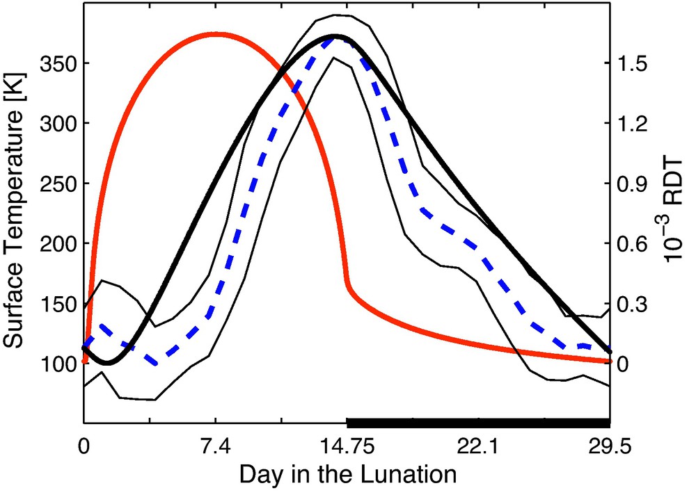
Results of the thermal model calculations for one lunation from sunrise to sunrise. Dashed curve: stack of the measured relative delay time variations from the eight lunations. Thin lines indicate the standard deviation. Continuous curves show model predictions for the relative delay times (black) and surface temperature (gray/red) (from Sens-Schönfelder and Larose, 2008).
Résultats des modèles de transports thermiques pour une période lunaire, d’aube à aube. Ligne brisée: mesures de variations relatives de délais moyennées sur huit jours lunaires. Les lignes fines indiquent l’écart type. Les courbes en traits continus présentent les prédictions théoriques pour les variations relatives de délais (noir) et la température du sol (gris/rouge) (selon Sens-Schönfelder and Larose, 2008).
Another observation that supports a relation between the RDT variations and heating by the sun concerns the amplitudes of the peaks of the RDT. They vary systematically from one lunation to another. The peak in January 1977 is about 20% higher than the peak in September 1976 (see Fig. 12). This variability can be qualitatively explained by variations in the sun-moon distance and energy inflow due to the eccentricity of the Earth’s orbit. The qualitative course of the energy inflow at noon is shown by the dashed curve in Fig. 12. It is in agreement with the changes of the RDT peak amplitudes.
Using 30 years old Apollo seismic data from the moon, we show that seismic waves in the crust are periodically slowed down. The shape of these delays and their periodicity indicate that they result from heating by the sun. Even variations of energy inflow due to changes in the sun-moon distance can be seen. The delay time variations reflect changes in the temperature profile of the lunar crust such that increased temperature lowers the seismic velocity. We propose a theoretical prediction for the temperature variation of the lunar subsurface that reproduces experimental variations.
6 Conclusions
In this article we discussed possible causes of subsurface velocity variations and presented the noise based technique to observe these changes. Three case studies were presented that demonstrate the range of applications for this technique. Velocity variations were shown to be caused by changes of the ground water level at Merapi volcano, by co-seismic effects in a fault zone in Japan and by temperature variations in the lunar subsurface. These investigations show that there is a variety of mechanisms that influence the subsurface velocity. In some cases it may be unclear which is the dominant effect. One question is the origin of co-seismic velocity changes in fault zones. Damage of near surface material would inhibit any type of pre-seismic signal whereas stain related velocity changes would at least in principle allow to observe the pre-seismic stress build-up. A key role in answering these questions will be played by techniques to locate changes in the medium that have to be developed in the future.
1 correlation of horizontal components oriented along the connecting line of the stations c.f. (Paul et al., 2005).
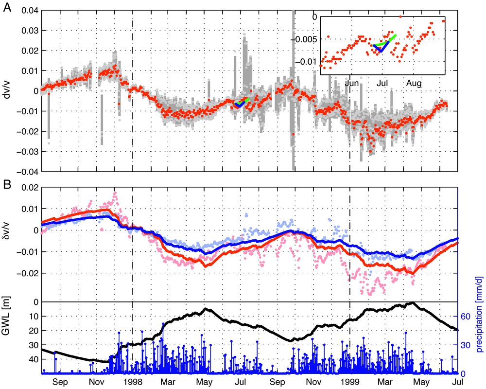
Measured and modelled velocity variations at Merapi volcano. A: Red dots mark the measurements in the 2–8 s time window. Individual measurements in the 2–4 s, 4–6 s, and 6–8 s seconds lapse time windows and their standard deviation are indicated by light gray dots and gray shading respectively. Results of the active CWI experiment (Wegler et al., 2006) are indicated by green and blue lines. B: Bottom part: daily precipitation rate (blue) and modelled ground water level (black). Top part: measured (light red dots) and modelled (dark red line) velocity variations in the 2–4 s time window. Same for the 6–8 s time window in blue (from Sens-Schönfelder and Wegler, 2006). Masquer
Measured and modelled velocity variations at Merapi volcano. A: Red dots mark the measurements in the 2–8 s time window. Individual measurements in the 2–4 s, 4–6 s, and 6–8 s seconds lapse time windows and their standard deviation are indicated by light gray ... Lire la suite
Variations de la vitesse mesurées et modélisées, au volcan Merapi. A: Les points rouges marquent les mesures effectuées dans la fenêtre de temps de 2–8 s. Des mesures particulières ont été effectuées dans des fenêtres d’intervalle de temps de 2–4 s, 4–6 s, 6–8 s et leur déviation standard est indiquée par des points gris et une zone ombrée respectivement. Les résultats de l’expérience active CWI (Wegler et al., 2006) sont indiqués par des lignes vertes et bleues. B: Partie inférieure: taux de précipitations journalier (bleu) et niveau d’eau souterraine modélisé (noir). Partie supérieure: variations de vitesse mesurées (points rose) et modélisées (ligne rouge foncé), dans la fenêtre de temps 2–4 s. Même chose pour la fenêtre de temps 6–8 s en bleu (selon Sens-Schönfelder and Wegler, 2006). Masquer
Variations de la vitesse mesurées et modélisées, au volcan Merapi. A: Les points rouges marquent les mesures effectuées dans la fenêtre de temps de 2–8 s. Des mesures particulières ont été effectuées dans des fenêtres d’intervalle de temps de 2–4 s, 4–6 s, ... Lire la suite