


 CC-BY 4.0
1. Introduction
The damage state of rocks in a fault core is a controlling element of seismic rupture and of the characteristics of fault evolution [Lyakhovsky et al. 1997; Cappa et al. 2014]. The interaction between slip and damage processes is poorly understood, especially as the nature and actual level of rock damage at depth are also poorly known despite some recent studies [Delorey et al. 2021]. On a geological time scale (i.e., over several seismic cycles), fault zones evolve, with the development of damage structures in their vicinity, partly due to dynamic stresses during rupture [Chester 1993]. The existence of this damaged zone is traditionally shown at depth by seismic tomography, which indicates a lower velocity zone that extends several kilometers in depth [Zigone et al. 2015; Roux et al. 2016; Allam et al. 2014]. More recently, it has been shown that the existence of a several kilometers thick zone of strong scattering around the North Anatolian Fault is required to explain the regional distribution of multiply scattered coda wave energies [van Dinther et al. 2021]. Passive scatterer imaging was made possible by a novel aberration correction method [Touma et al. 2022] that confirmed the presence of intense fracturing at depth around the San Jacinto fault in California.
Indeed, measurements of the temporal evolution of seismic wave velocities give information on the mechanical state of the medium [Poupinet et al. 1984; Schaff and Beroza 2004; Langlois and Jia 2014]. Noise-based passive monitoring allows to envision long-term continuous monitoring of the seismic velocity [Brenguier et al. 2008, 2014; Sens-Schönfelder and Wegler 2006; Rivet et al. 2014]. Examples of these changes are now well documented, and it is possible to detect them continuously with unprecedented precision that can reach a few 10−5 for relative velocity changes [Wang et al. 2017] and very short time resolution [Mao et al. 2019b; Sens-Schönfelder and Eulenfeld 2019].
One difficulty with these measurements is to distinguish between changes related to internally induced deformations and changes related to external forcing, such as precipitation [Sens-Schönfelder and Wegler 2006; Barajas et al. 2021], temperature [Meier et al. 2010], or tides [Sens-Schönfelder and Eulenfeld 2019]. As the causes of external forcing are fairly well known, correction strategies have been proposed [Wang et al. 2017]. Assessing these changes in the vicinity of rupture zones will improve through the development of sensitivity kernels for spatial inversion methods [Margerin et al. 2016; Obermann et al. 2016; van Dinther et al. 2021; Barajas et al. 2021; Zhang et al. 2021].
With the striking increase achieved in quantity and quality of seismic observations and the novel methods now possible, a way is opening to revisit the vision of earthquake processes. At the same time, geodetic measures reach impressive precision. At time scales from days to years, evidence for changes in elastic moduli in response to earthquakes [Brenguier et al. 2008] and transient tectonic deformations [Rivet et al. 2014] has been shown in the form of a velocity drop followed by a slow recovery similar to laboratory observations [TenCate et al. 2000]. These changes are also observed at the time scale of days in a mining environment [Olivier et al. 2015] and in laboratory experiments of stick-slip and slow slip [Scuderi et al. 2016], where a drop in the elastic moduli starts even before the slip is observed.
Such effects have been largely studied in rocks with laboratory experiments. They have revealed that the application of a uniaxial stress involves elastic wave velocity anisotropy [Nur and Simmons 1969] that could be linked to the elastic nonlinear behavior of rocks [Johnson et al. 1996; Johnson and Rasolofosaon 1996; Pasqualini et al. 2007]. Direct comparisons between rock degradation (linked to a damage quantified by the distribution of microcracks) and wave velocity measurements could be highlighted experimentally [Hamiel et al. 2009]. Furthermore, theoretical considerations based on the inversion of the measured wave velocities and resulting microcrack density tensors allowed to describe the microcracks evolution and anisotropy [Sayers and Kachanov 1991, 1995; Schubnel and Guéguen 2003; Stanchits et al. 2006; Hall et al. 2008]. For the following numerical simulations, we consider granular materials rather than real rocks as they have been studied as synthetic rocks in previous experiments [Langlois and Jia 2014; Canel et al. 2020].
An important issue is to explain how the very small macro-scale deformation that is associated with tectonic deformation can induce an observable velocity drop. In this study, we focus on the drop effect without consideration of the slow logarithmic type relaxation effect [TenCate et al. 2000] observed in the earth after a strong drop [Brenguier et al. 2008].
Here we use a simple cemented granular media model [Dvorkin et al. 1994; Langlois and Jia 2014; Hemmerle et al. 2016] to represent the behavior of rocks around faults that are intensely fractured and cemented by precipitation due to fluid transfer. Our interest in this simulation is to link it to the observed temporal variations of seismic wave propagation velocities. More precisely, in the following, we use numerical simulation models to analyze the relation between the wave velocity drop and the damage evolution. We focus on numerical simulations in an edometric experimental setup, such that some comparisons with real experiments can be done. The edometric experiment is a typical experiment in soils and granular materials [Evesque 2000; Sawicki and Swidzinski 1995; Langlois and Jia 2014], which involve macroscopic deformation of up to 15%. In the first stage, the goal is to deform and damage a medium in which we will later study wave propagation [Langlois and Jia 2014]. Only small overall deformation (up to 1.5%) will be considered here. However, as even for small macroscopic strain the microscopic bond deformation is large and very heterogeneous, large deformation modeling will be considered at the microscopic scale.
The numerical granular material considered in this paper is made from a dense elastic bead packing that includes some cement. The numerical simulations can highlight the microscopic heterogeneities. For this we used the finite element method, instead of the discrete element method [Radjai and Dubois 2011], and we meshed both the beads and the bonds. As far as we know, this approach has not been used in granular modeling. In contrast with the discrete element method approach, which is widely used in granular physics, the finite element method approach provides a fine description of the damage mechanism at bonded contacts and of the elastic wave propagation through the bonds and the particles (beads).
To limit the computational load, we consider only two-dimensional (2D) numerical simulations. The mechanical modeling of the bonds relies on a simple elasto-plastic model with damage, while the beads are assumed to be elastic and isotropic. Following the edometric experimental setup, we first detail the adopted geometry for the cemented granular material, and then we distinguish two processes in the following sections. The first process is quasi-static loading of the heterogeneous macroscopic sample that involves damage to the bonds. This first modeling aims at creation of a realistic state of deformation at the microscopic scale. The second modeling is the dynamic propagation of a small perturbation in a linear elastic regime for a given state of damage of the material. This second process can be considered as the dynamic version of the “tangent problem” associated to the quasi-static evolution. It represents the actual situation encountered in geophysical monitoring of active faults: an elastic, weak amplitude wave propagates in a medium where damage results from a slow internal deformation. Note that the macroscopic damage of the sample, which is defined from the variation of the macroscopic elastic coefficients, cannot be found from the strain–stress curve obtained from quasistatic unidirectional loading. For this, we would need several unloading/reloading experiments. The macroscopic damage is therefore probed by the wave propagation, as in the seismological measurements of the wave speed.
2. Quasistatic loading
2.1. Macroscopic setting
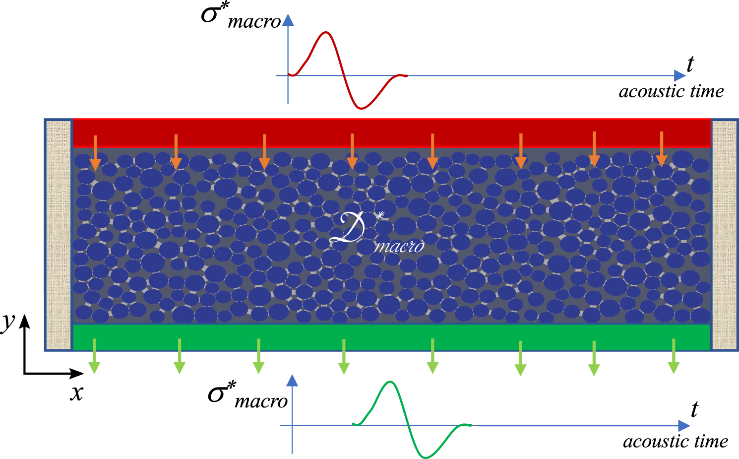
Let us first describe the numerical edometric experiment. The “sample” (or cell) of the cemented granular material initially occupies the 2D domain
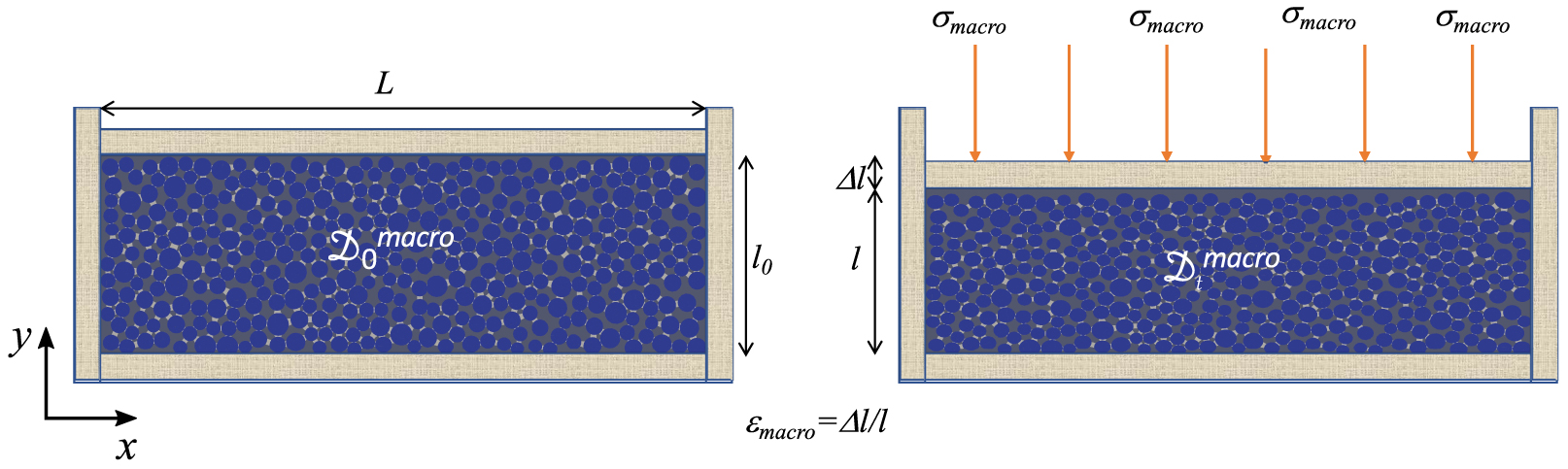
Representation of the quasi-static edometric numerical experiment.
2.2. Microscopic setting
The cemented granular material, which occupies at the moment t ∈ [0,Tquasi-static] the domain
After creation of the packing, we checked that the bonds are isotropically generated, so as not to induce any geometric anisotropy from the fabric that might hide or perturb possible anisotropic effects due to the future quasi-static loading. Figure 2b shows the polar probability distribution of the orientation angles of the bonds (i.e., angle between the (Ox) axis and the axis that connects the center of the beads, as schematized in Figure 2d). Half the polar diagram is shown, as it is π-periodic: each bond is indeed indexed on the basis of both its associated bead, with an angle 𝜃, and the other associated bead, with an angle 𝜃+π. The distribution is globally isotropic (a sample with more bonds would exhibit a smoother distribution).
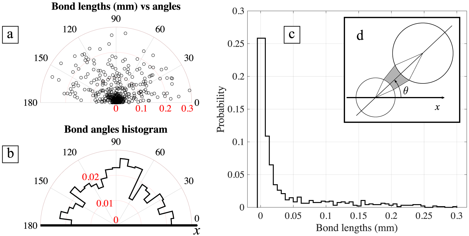
Geometric statistics of the initial isotropic packing. (a) Bond length as a function of the orientation angle of the corresponding bond. (b) Polar probability distribution of the orientation angles of the bonds. (c) Probability distribution of the lengths of the bonds. (d) Definition of the orientation angle 𝜃 of a bond.
Figure 2c shows the distribution of the length of the bonds, defined as the distance between the centers of the beads concerned and the sum of their radii; this then represents a length along the bond symetrical axis. The minimal values correspond to the closest beads and tend towards zero, as there is no minimal limit for the generation of bonds in the sample considered. The majority of the bonds have a length less than 0.05 mm.
Further geometric anisotropy can come from correlations between the lengths and the orientations of the bonds. Indeed, as we expect that short bonds are more affected by the macroscopic deformation, we verified that there is no privileged direction for them. Figure 2a shows the lengths of the bonds as functions of the orientation angles of the corresponding bonds in a polar plot. The isotropic distribution shows that there is no correlation between length and orientation angle.
2.3. Mechanical modeling
For the mechanical modeling of the bond material, which is detailed in Appendix, we chose the model of Lemaitre and Chaboche [Lemaitre and Chaboche 1994] coupling isotropic ductile plastic damage and with an elasto-plastic law in the framework of an Eulerian (large deformations) description [see for instance Belytschko et al. 2000].
For this, we considered the additive decomposition of the rate deformation tensor in the elastic and plastic rates of deformation. For the elastic range, we considered an isotropic hypo-elastic law (i.e., the large strain generalization of Hooke’s law with the Lamé coefficients 𝜆 and 𝜇 written in terms of the Jaumann rate of the Cauchy stress tensor and the elastic rates of deformation). The plastic rate of deformation is related to the Cauchy stress tensor through the flow rule associated to the classical Von-Mises yield criterion (without hardening). The weakening effect is characterized by a damage (phenomenological) parameter d ∈ [0,1] and its evolution law is related to the cumulated plastic strain 𝜖p.
The model parameters used here have not been characterized or calibrated experimentally. This important task is beyond the scope of present numerical study. However, the mechanical parameters have been chosen to correspond to a very ductile cement, as tetradecane or eicosane, that has been used in laboratory experiments showing seismic velocity reduction during compression [Langlois and Jia 2014; Canel et al. 2020]. The elastic coefficients of the undamaged material are given in Table 1 and the yield limit is 𝜅0 = 135 MPa. For simplicity, the dependence of damage rate on the cumulated plastic strain is given through a piecewise linear function. When the cumulated plastic strain reaches an activation level 𝜖p,activation = 2%, we consider the beginning of damage process, while the maximal level of damage is dmax = 0.8 corresponding to 𝜖p,max = 20%.
Parameters for simulations
| 𝜌 (kg/m3) | E0 (GPa) | 𝜈0 (GPa) | M0 (GPa) | cp0 (m/s) | cs0 (m/s) | |
|---|---|---|---|---|---|---|
| Beads | 2600 | 60 | 0.24 | 70.72 | 5200 | 3100 |
| Bonds | 1200 | 3.5 | 0.33 | 5.18 | 2100 | 1000 |
The index 0 refers to the state without damage.
The beads material was supposed to be purely elastic (see Table 1 for the Lamé coefficients corresponding to glass), with no damage effects or plastic strains. This choice could appear too simple but corresponds to a granular material made from glass beads used in laboratory experiments for which no bead crushing has been observed [see for instance Langlois and Jia 2014; Canel et al. 2020]. Moreover, this choice allows us to focus on the bond material, and to analyze the crucial role played by the bonds damage in the wave velocity drop. This is due to damage localization in the bonds, which are pointed out in the next numerical results obtained with the choice of damage parameters presented above. The presence of a maximal level of damage in the model prevents total bonds failure (that would be very difficult to handle in an elasto-plastic FE computation of a large number of bonds) but is not expected to affect the overall results at the low levels of macroscopic deformation at which we limit our simulations.
2.4. Numerical modeling
As the bonds are submitted to large deformation (even for small macroscopic deformation), we used an arbitrary Lagrangian Eulerian (ALE) description [Huerta and Casadei 1994; Wang and Gadala 1997; Ghosh and Raju 1996; Rodríguez-Ferran et al. 2002]. This description incorporates the advantages of the Lagrangian and Eulerian descriptions, and can avoid some of their drawbacks. Usually in solid mechanics, where we do not deal with large mass fluxes among different parts of the sample and the strains are not too large, the Lagrangian kinematics formulations are intensively used. However, because of severe distortion of elements in some practical problems, the determinant of the Jacobian matrix can become negative, which results in numerical errors. Eulerian methods coupled with an ALE description (which either uses a fixed mesh or adapts the mesh at each time step) can eliminate the problems associated with distorted meshes. With the ALE method adopted here, the computational grid can be moved arbitrarily, to optimize element shapes independently of material deformation.
For the numerical integration of the equilibrium of the hypo-elastic-plastic model described above, to find the Eulerian unknowns acting on the domain
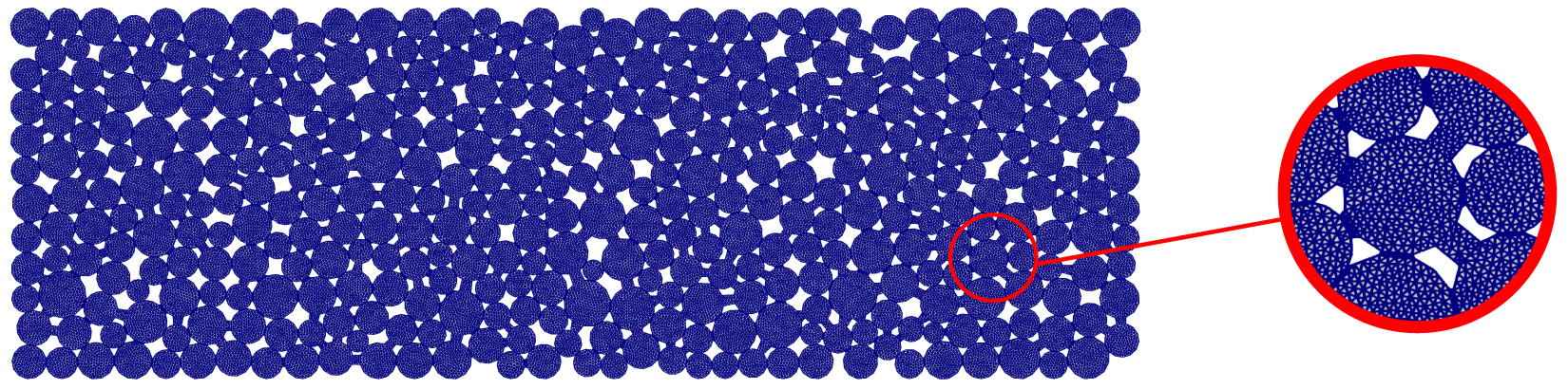
Since the investigated processes are very different, the quasi-static and dynamic problems require two distinct meshes (one can see the difference by comparing Figures 3 and 8). For the quasi-static problem, as the beads are almost not deformed outside of their peripheral zone, it is not necessary to mesh them finely at the core, but only close to the bonds that need a fine mesh to correctly describe their large deformation. The initial mesh is then finer in the bonds and the periphery of the beads, with a given ratio between the size of the edges (see Figure 3). Moreover, to capture the shear bands, we used an adaptive mesh technique with respect to the plastic strain rate norm | Dp|. This means that regions where the plastic strain rate is larger will have a fine mesh, while elsewhere the mesh is coarse. The ratio between the sizes of the fine and coarse meshes was 1∕4.
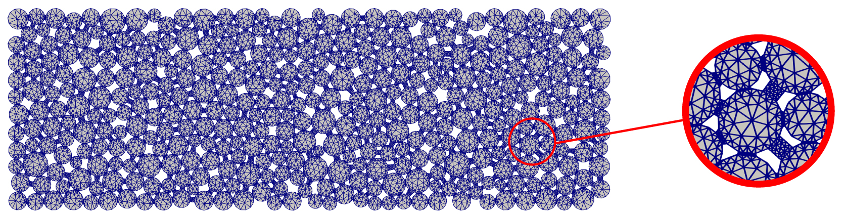
The initial mesh used for the quasi-static computations.
2.5. Results
2.5.1. Macroscopic level
Figure 4 shows the macroscopic normal load 𝜎macro versus the imposed strain on the sample 𝜀macro. The macroscopic load initially increases linearly with the displacement, which highlights an elastic behavior. The linear fit close to the origin (see Figure 4) gives an estimation of the initial (undamaged) macroscopic uniaxial strain modulus (P-wave modulus)
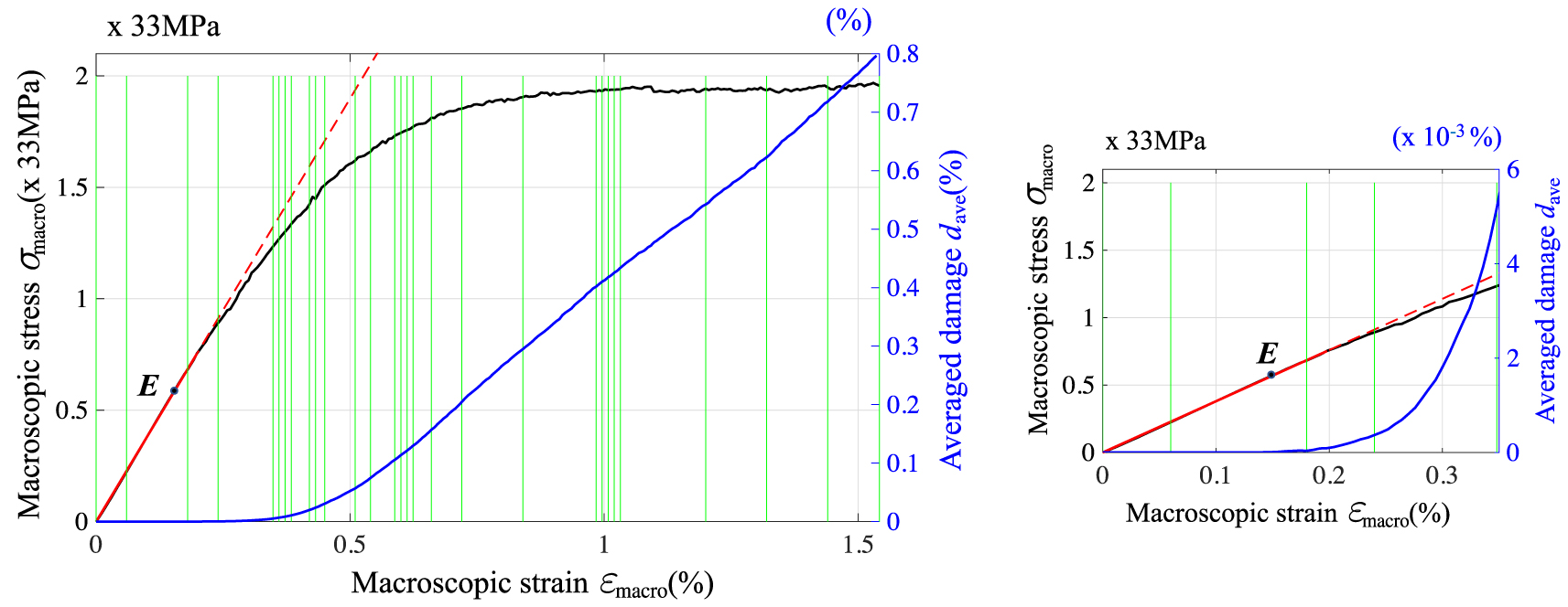
(a) Macroscopic stress 𝜎macro (black; in × 33 MPa) and the averaged damage dave (blue; in %) as functions of the strain 𝜀macro (in %). A linear fit of the load (red) highlights its first elastic trend. The chosen states for the dynamic computations are indicated with vertical green lines. (b) Zoom in around the low strains.
However, the macroscopic damage dmacro of the sample, defined as
This kind of quasi-static unloading/reloading experiments with fluid pressure are possible at the laboratory scale or at a small geophysical scale corresponding to reservoirs for example (in the framework of the oil and gas industry). However, as far as we know these techniques have never been applied in Nature to a fault zone at the scale relevant to earthquake studies. One can think about the tides effect but our study does not target it. Indeed, different techniques have been used to study the tide effect and actually highlighted the velocity dependence on tide deformation independently from the presence of a fault system [Sens-Schönfelder and Eulenfeld 2019; Mao et al. 2019a; Reasenberg and Aki 1974; Takano et al. 2014; Delorey et al. 2021]. Nevertheless, the continuous nature of tides implies that they are not a source of evolution damage, or over time scales and amplitudes that are incompatible with their measurements. In our perspective, non-linearity and damage evolution are quite different. This is why we did not use the quasi-static unloading/reloading technique to measure the macroscopic damage but the wave speed probing (see next section), which is much more adapted to the targeted geophysical measurements.
We computed and plotted the microscopic averaged damage dave(t), defined as the ratio between the integral of the damage, that vanishes outside the bonds, and the area of the sample
2.5.2. Microscopic level
Even for small macroscopic deformation, local plastic irreversible deformation occurs in the bonds. The first microscopic plastic and damage effects occur at 𝜀macro = 0.096% and 𝜀macro = 0.132%, respectively (see Figure 4 for the damage). This is consistent with the chosen microscopic laws with successive plastic and damage thresholds (see Section 2.3 and the Appendix for more details). The damage process is very heterogeneous as it occurs along the force chains. Some of the bonds are not damaged, and some of them are completely damaged, although there are a lot of bonds in an intermediary state where the damage is localized in microscopic shear bands. We note that there is no macroscopic localization of the damage (i.e., no noticeable development of a macroscopic shear band).
Figure 5 shows the deformed configuration at the end of the edometric numerical experiment (
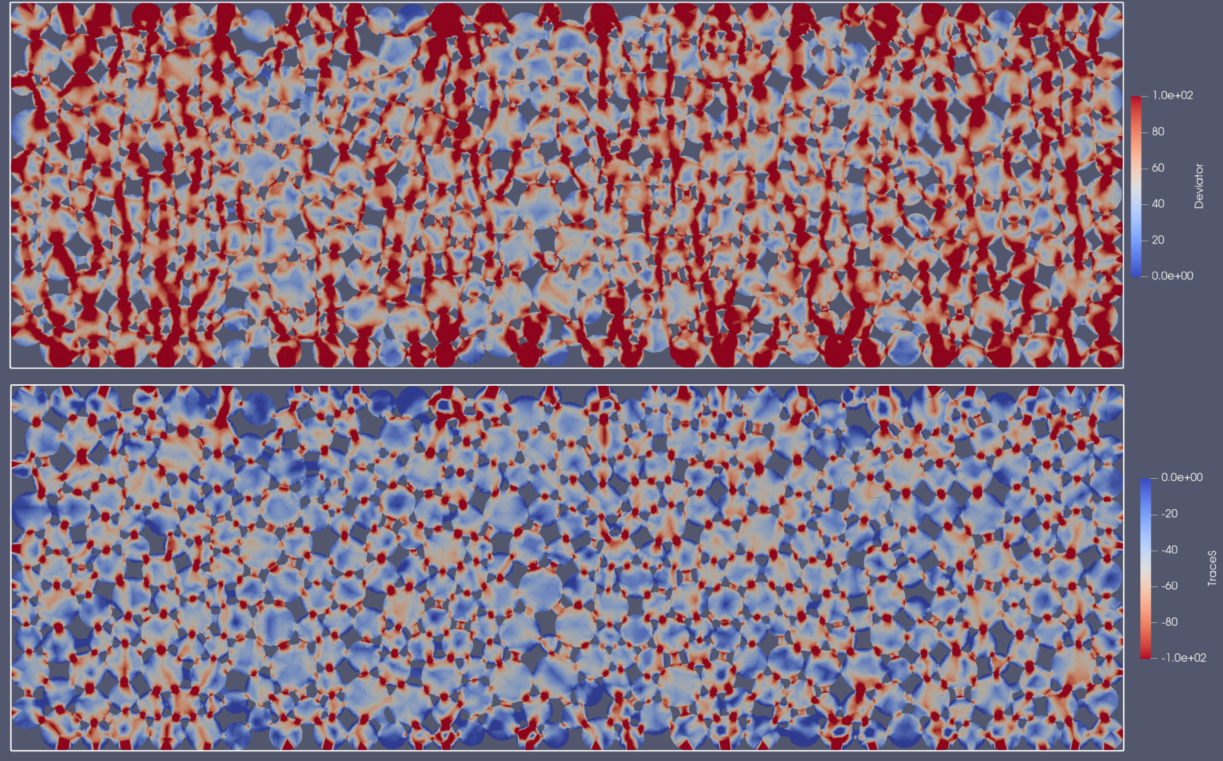
Top: Map of the (Von-Mises) equivalent stress (in MPa) that describes force chains in the cemented packing at the final stage of compression. Bottom: Map of the mean stress (in MPa).
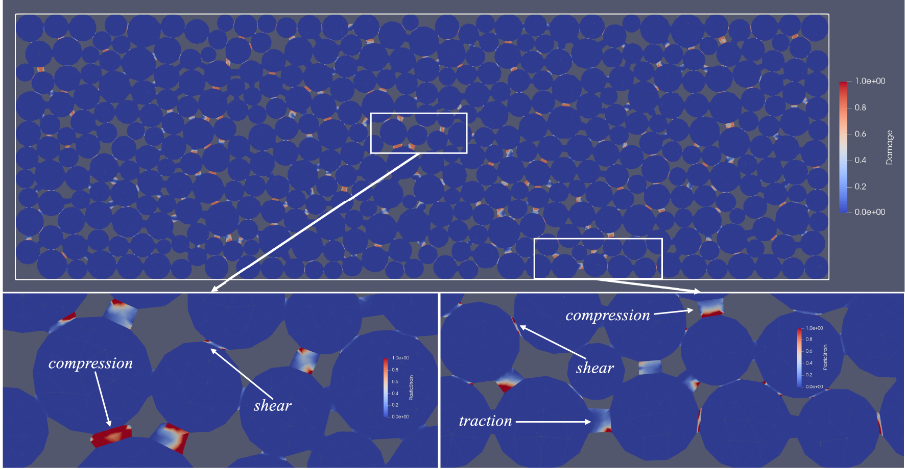
Top: Map of the damage distribution at the final stage of compression. Bottom: Zoom in boxes with the cumulated plastic strain on a color scale.
Even at this low level of compaction we found that new contacts between the grains and the walls are established, but no new contact between the grains appear during the loading. That means that the P-wave propagation is not facilitated by these new inter-grains contacts as discussed in the context of “non-classical nonlinearity” or “clapping interface model” [Chaboche 1992; Lemaitre and Desmorat 2005; Pecorari and Solodov 2006; Lyakhovsky et al. 2009].
3. Elastic wave probing
In this section, we present the simulations of the wave propagation, to highlight the wave speed sensitivity to the damage state of the sample. We want to show that it is possible to monitor the macroscopic damage through the wave speed record. For this, we model the propagation of small amplitude, purely reversible, non-destructive waves in the damaged material at different stages of the quasi-static loading. These stages are chosen to better understand the impact of large and small increments of damage and different regimes of the loading process (i.e., elastic at the beginning, then inelastic with increased damage).
3.1. Problem setting
3.1.1. Macroscopic level
At different stages
Representation of the ultrasound probing numerical experiment.
Note that in the seismological context, and for fault monitoring, the seismic velocity monitoring relies on relatively low frequency waves (less than a few Hz) due to the rapid attenuation of the waves in the complex, highly fractured rocks of the fault core. This mean that the probe has a wavelength much larger than the typical grain size.
The macroscopic computations of the P-wave speed
| (1) |
3.1.2. Microscopic level
At different stages of the quasi-static loading process described in the previous section, and as indicated by green vertical lines in Figure 4, we stored the deformed meshes and the damage distributions. Let us denote the domain occupied by the cemented granular material by
3.2. Mechanical and numerical modeling
As the waves have a small amplitude, there is no evolution of the damage and plastic strain during the dynamic process, which is said to be nonperturbative or nondestructive. This is why the small perturbation assumption can be considered to be valid and the material can be supposed to be linear elastic, with the mass density 𝜌∗ and the elastic coefficients 𝜆∗, 𝜇∗, given by
The dynamic problem is discretized in time by the classical implicit Newmark method, with 𝛽 = 1∕4 and 𝛾 = 1∕2 [e.g., see Fung 1997], which is unconditionally stable and thus allows much larger values of the time step than the critical Courant–Friedrichs–Lewy time step. For the space discretization, we used [P2-continuous] finite element discretization for the displacement field and [P1-discontinous] for the stress field.
The quasi-static mesh used previously is not appropriate for wave propagation. For the dynamic wave propagation simulation, the domain
The initial mesh used for the dynamic computations.
3.3. Results
The low-frequency pulse (for which the wavelength in the glass is almost 50 times the mean radius of the beads) generates a well-established coherent wave, without remarkable multiply scattered waves. It is visible at t = 2 μs after the excitation in the first line of Figure 9, which shows several snapshots of the longitudinal stress 𝜎yy field in all of the sample. The left row shows the undamaged sample (
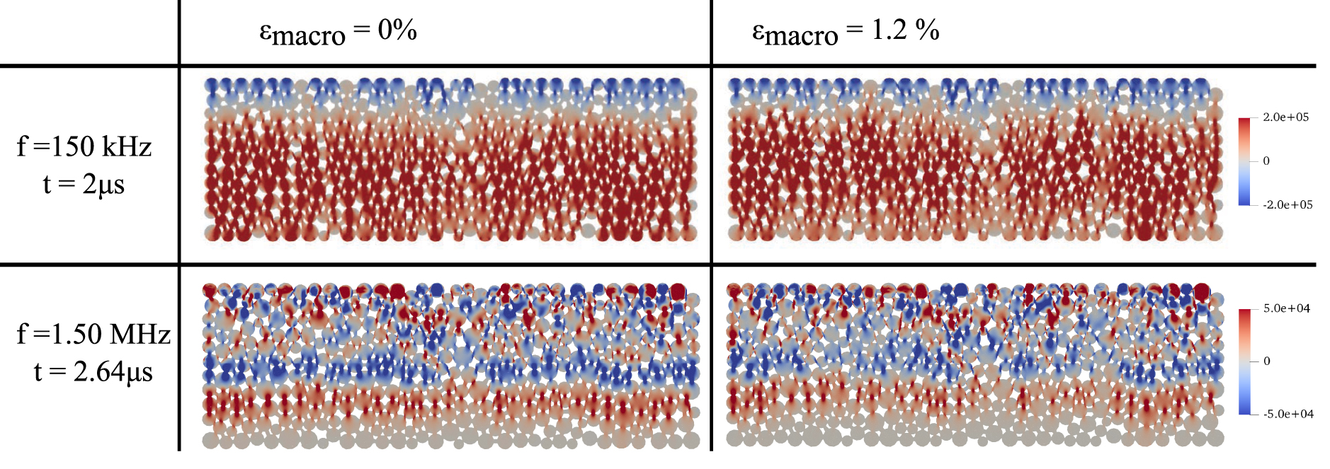
Snapshots of the longitudinal stress 𝜎yy field (as a color scale) at t = 2 μs after the low-frequency excitation (top) and at t = 2.64 μs after the medium-frequency excitation (top), in the undamaged sample (left) and after compression (right) corresponding to
Snapshots of the longitudinal stress 𝜎yy field (as a color scale) at t = 2 μs after the low-frequency excitation (top) and at t = 2.64 μs after the medium-frequency excitation (top), in the undamaged sample (left) and after ... Lire la suite
For the 1.50 MHz pulse (for which the wavelength in the glass is almost 5 times the mean radius of the beads), a similar delay can be observed between clear coherent waves computed with the undamaged state and the same damaged state, as seen in the second line of Figure 9. However, in this case, the coherent waves are followed by multiply scattered waves, producing a tail in the signal similar to the seismic coda. Note the complexity of the field distribution at both the macroscopic scale and the bead scale, due to the high heterogeneity of the granular material.
The transmitted 𝜎yy-waves are recorded along the bottom wall (called the “reception wall”), as discretized in 1000 spatial points and shown for the 1.5 MHz pulse in Figure 10. They are gathered when they belong to the same bead of the reception side, making voids appear between the 26 beads of this side. One of these signals is plotted in Figure 11 (in green) for different states of damage of the sample. The sum of all these signals is visible as the blue curve inside the right box of Figure 10, which enhances the coherent arrivals. Indeed, unlike the coherent wave that is almost uniform along the y-axis, the codas depend on the recording position. So their sum, which is physically defined in the experiments by the large transducer in contact with all of the beads of the reception wall, tends to cancel, whereas the summed amplitudes of the coherent wave and its reflections are enhanced.
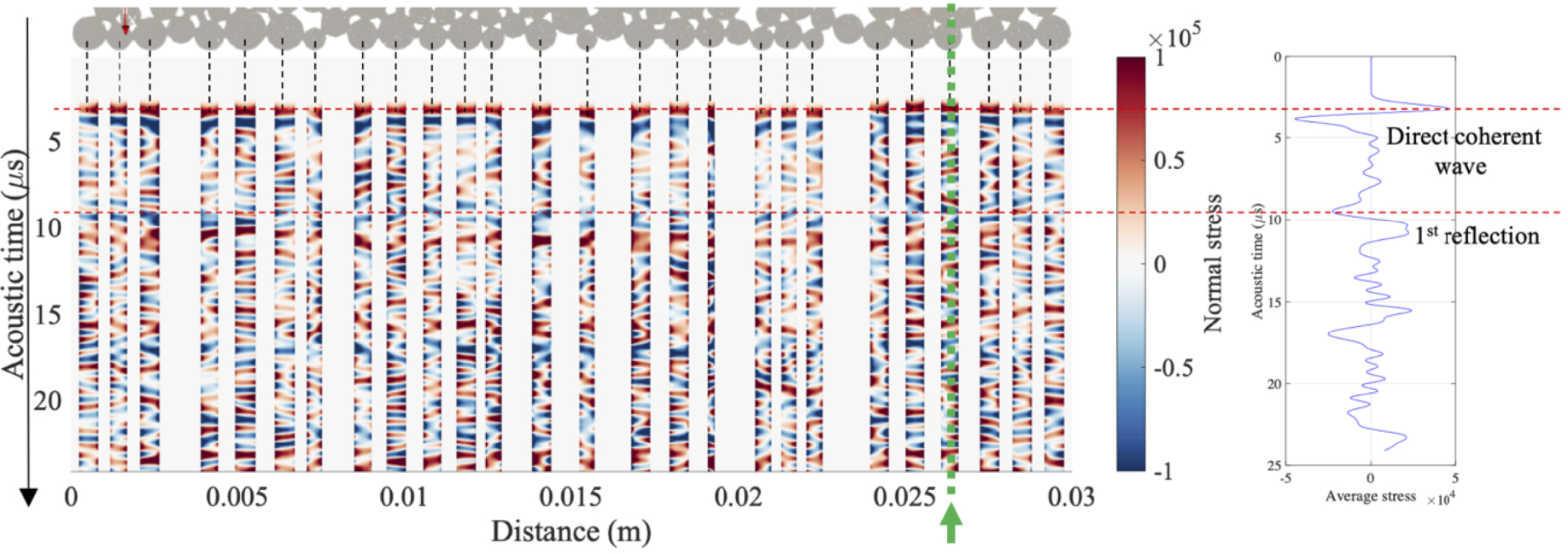
(a) Acoustic signals recorded along the reception wall (represented above) for a 1.5 MHz pulse. The green arrow indicates the position chosen to compare the codas in Figure 11. (b) Summed waves along the reception wall.
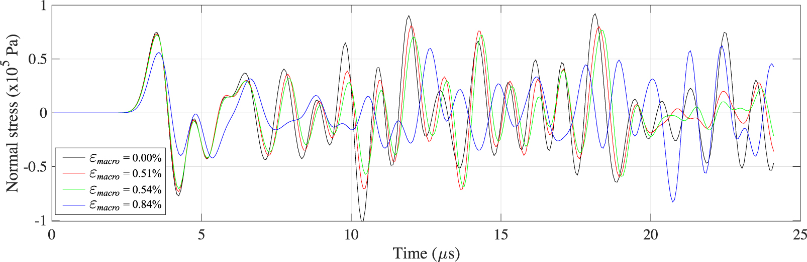
The transmitted acoustic signals recorded for a 1.5 MHz pulse at the same position of the reception wall (indicated in green in Figure 10) for the undamaged sample (black) and after different steps of compression: 𝜀macro = 0.51% (red), 𝜀macro = 0.54% (green), and 𝜀macro = 0.84% (blue).
The signals plotted in Figure 11 are associated with different levels of damage as they correspond to the macroscopic strains 𝜀macro = 0%, 𝜀macro = 0.51%, 𝜀macro = 0.54% and 𝜀macro = 0.84%. We observe that the second and third signals in Figure 11 are very similar, which is understandable, with the weak strain and the damage difference between them. The third signal in Figure 11 is slightly delayed compared to the second one, with a small amplitude loss, and this delay increases visibly with the acoustic time t between 7 and 20 μs. After 20 μs, these signals are not coherent anymore. Similar, but more pronounced, observations can be made between these two signals and the first one computed with the undamaged sample. We note that the first coherent peak, which corresponds to the direct transmitted ballistic wave, has almost the same amplitude and time of flight for these three signals. This is not inconsistent, as at the same time the thickness of the sample decreases and the wave velocity decreases. The contrast between the signals is much more obvious with the fourth signal computed, when the quasistatic loading begins to saturate after important damage to the sample. We observe a loss of amplitude of the transmitted ballistic wave and a time of flight increase. At later times, we observe important changes in the coda. These can be explained by the increasing scattering process of the waves due to two changes: the first one is the increasing impedance contrast between the glass and the damaged cement at the interface bead/bond linked to the degradation of the elastic parameters of the cement; the second one is the slight geometric evolution of the sample without true rearrangement, as the contacts remain the same (i.e., no loss, no creation).
The sum of the signals along the reception wall allows estimation of the time of flight of the transmitted pulse, and therefore of the velocity of the longitudinal coherent wave, as the ratio of the time of flight and the thickness of the numerical sample at the considered state of damage. We choose the time of flight measured from the first peak. The velocities obtained are shown in Figure 12 for the low-frequency pulse, to ensure that the coherent regime is well established, and validate the approximation of the effective medium theory [Digby 1981]. The velocity can also be calculated from the mean time of flight over the statistics of the signals recorded at 1000 positions along the reception wall, which gives very close results, as can be seen in Figure 14b for a 1.5 MHz pulse.
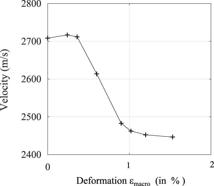
The wave velocity V in the sample during a quasistatic process versus the macroscopic strain 𝜀macro. The velocity is calculated with the time of flight of the summed signals along the reception wall for a low-frequency pulse (150 kHz).
Figure 12 shows that for a low frequency pulse (150 kHz), the velocity first increases slightly in the elastic part of the deformation, when there is no damage (dV∕V close to +1%); it then decreases dramatically (dV∕V close to −10%). The first phase is associated to a slight increase of the wave velocity and can explained easily on the basis that at the begining some additional disks enter into contact with the rigid piston, which creates new force chains that facilitate the wave propagation. The decrease in wave velocity begins when the bonds are damaged; i.e., when the microscopic damage average dave starts increasing significantly (see Figure 4). It is remarkable that a very small amount of microscopic damage average can imply such a dramatic loss. Moreover, when the load reaches its stationary value, the velocity keeps decreasing, although by less, despite the almost constant microscopic damage average rate
In all of these considerations, it appears clear that the microscopic damage average dave, defined as the ratio between the integral of the damage and the area of the sample
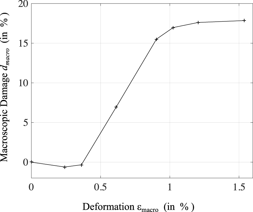
The macroscopic damage dmacro computed with elastic wave probing (with a low-frequency pulse of 150 kHz) versus the macroscopic strain 𝜀macro.
To check the validity of the velocities calculated with the time of flight in the case of a 1.5 MHz pulse, we use the doublet technique [Poupinet et al. 1984], which is also called the moving-window cross-spectrum technique [Clarke et al. 2011] or coda wave interferometry [Snieder et al. 2002]. We apply this to all the consecutive couples i − 1,i corresponding to the consecutive chosen quasistatic steps for the dynamical simulations. This ensures good temporal coherence between the signals i − 1 and i, as shown in Figure 11, which is necessary to apply this technique. This technique is especially interesting for subtle changes of the material velocity, and it consists of the evaluation of the relative velocity change 𝛿vij = (vj − vi)∕vi of the medium at a given position between two temporal states i and j. We can also write 𝛿vij =𝛿 lij −𝛿 tij with 𝛿lij linked to the strain (calculated from the quasistatic loading), 𝛿tij = dtij∕t as the relative change of the time of flight dtij of the wave through the sample, and t as the acoustic time, which is zero at the beginning of the excitation pulse. The procedure to evaluate 𝛿tij has two steps: calculation of dtij(t) for different times t in the whole range of the acoustic time (so with the ballistic parts and the codas), as sufficient for the second step, which is linear regression of dtij with t. This regression goes through the origin and its slope is directly 𝛿tij. Figure 14a shows the two contributions 𝛿lij(t) and 𝛿tij(t) as functions of the macroscopic deformation. The two contributions were calculated between consecutive pairs i − 1,i and were accumulated, to be compared to the initial step 0. The cumulative error from the last regression of the doublet technique is also plotted in Figure 14a. It increases with the macroscopic deformation, until almost 0.5% at the last step, as the nondeformed configuration is taken as the reference here.
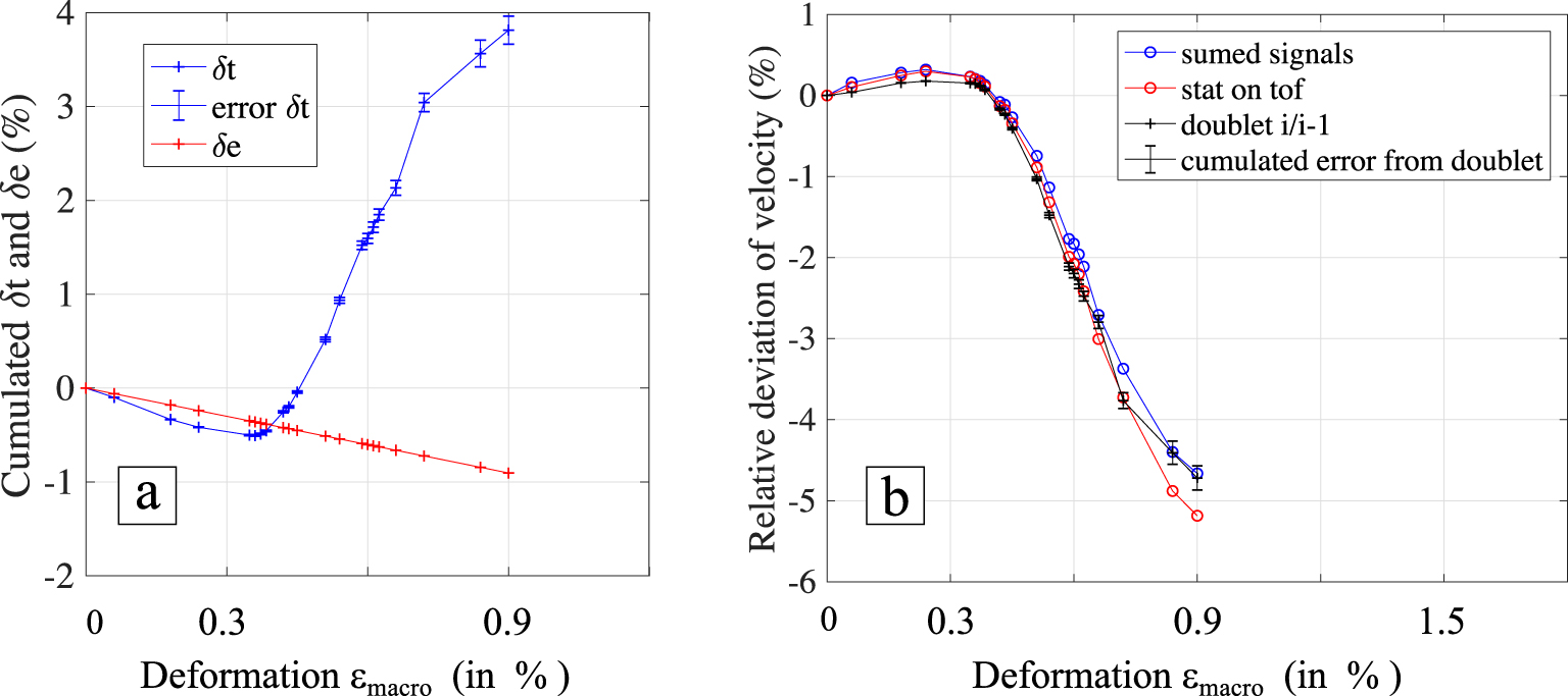
Velocity changes computed with the doublet technique for a 1.5 MHz pulse. (a) Thickness (red) and delay (blue) changes as functions of the quasistatic step. Error bars on the delay come from the last regression of the doublet technique. (b) Velocity changes as a function of the quasistatic step and computed with the doublet technique (black), from the time of flight statistics (red) and the time of flight of the summed signals (blue).
Figure 14b shows the velocity change 𝛿vij(t), which is the difference between these two contributions. The same error bars are also plotted. The velocity changes obtained with the times of flight and both of the summed signals and from their statistics (from the same dynamic simulations) are also plotted here. The results are very close.
4. Induced damage anisotropy
In this section, we investigate how the induced damage is related to the loading direction. We also investigate the loss of isotropy of the macroscopic wave propagation. As the effects are similar and more pronounced in the x-axis than in the y-axis direction, we consider the quasistatic edometric compression along the x-axis. For this simulation, the final strain is 𝜀macro = 2.17%.
The “norm” of the deviatoric stress tensor is shown in Figure 15a, which corresponds to the last step of the computation. It shows that the force chains tend to be oriented along the axis of the loading. This assumes that the bonds oriented along this same axis are more solicited for the transmission of the stress, and as a consequence they would be more damaged than the others. This can be seen in Figure 15b, which shows the distribution of the damage parameter d in the bonds at the last step. To rigorously demonstrate this observation, Figure 15c shows the value of the damage integrated over each bond independent of the others, as a function of its angle. Clear anisotropy appears and confirms the previous hypothesis: the damage is concentrated in the bonds with angles in [π∕6;5π∕6] modulo π.
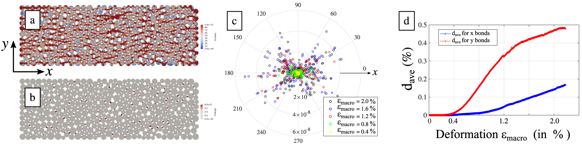
Edometric compression along the x-axis. (a,b) Maps of the deviatoric stress and damage parameter d, respectively, at the last step of the quasi-static computation. (c) Damage integrated over the bonds independently as a function of their angle for different macroscopic strains. (d) Damage integrated over the “x-bonds” and “y-bonds” as a function of the macroscopic strain.
Therefore we define the “x-bonds” and “y-bonds” as the two groups of bonds with angles between [−π∕6;π∕6] and [π∕3;2π∕3] modulo π, respectively. Figure 15d shows the values of the damage
These computations on the damage average suggest that the bounds orientated along the propagation axis are mainly implied in the speed wave drop. To confirm this assumption, we can test the anisotropy of the wave propagation by measuring the wave velocity along the x-axis and y-axis (called Vx and Vy, respectively) in the configuration of this section with compression along the x-axis. We use low frequency pulses (150 kHz), as defined in Section 3, at six different steps of the same quasi-static compression simulation. With the associated wavelength of 20 mm, we consider that no multiple scattering occurs, which would considerably change the comparison between the two axes, as the wall is three times longer than the other one and would accumulate more scattering effects. The velocities are plotted in Figure 16 and are computed with the time of flight of the first peak of the summed signals recorded along the corresponding wall and the thickness (constant for the propagation along the y-axis).
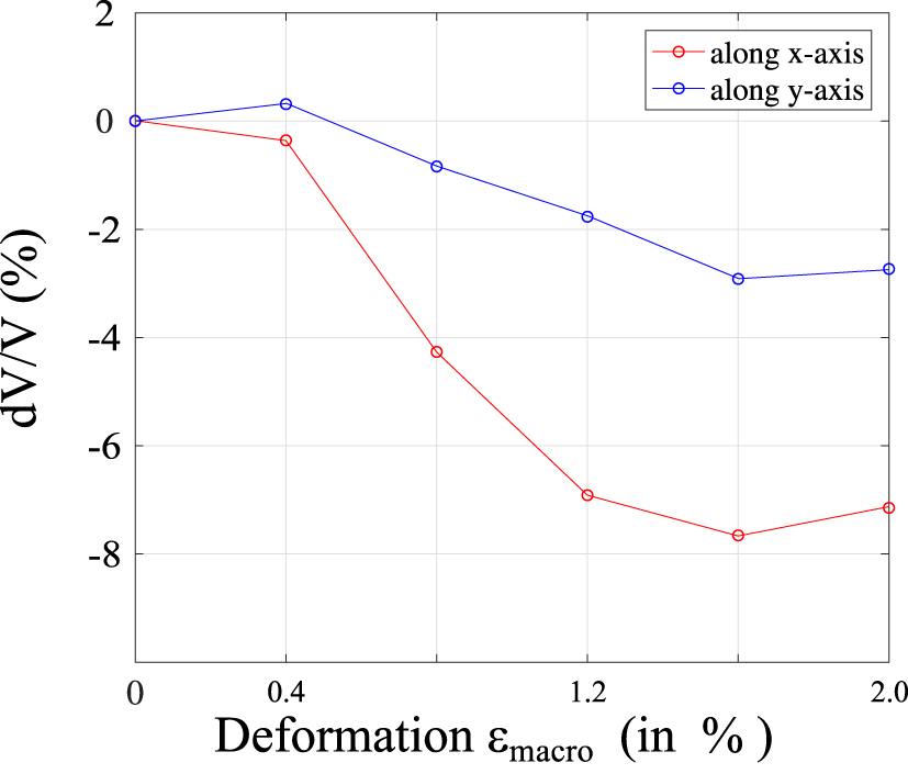
dVx∕Vx and dVy∕Vy divided by their respective initial values as functions of the macroscopic deformation. The velocities are calculated with the time of flight of the summed signals along the reception wall for a low-frequency pulse (150 kHz).
First, we check that Vx and Vy are almost the same at the initial state without compression (step 0), as there should not be any source of anisotropy at this step. We indeed find values that are close, as 2740 and 2690 m/s respectively, with a relative deviation of 1.8%. The small difference might be due to the geometry of the sample and the boundary conditions. Then we observe that both velocities are impacted by the loading and the induced damage, even Vy, and where Vx shows a decrease of 7%, twice the decrease of Vy. This confirms the induced damage anisotropy for the wave propagation.
As they are calculated with the same method, we can also compare Vx and Vy to V , the velocity obtained from the compression and the wave propagation along the same y-axis represented in Figure 12a. V and Vx are very similar, with very close values and the same trend for 𝜀macro between 0.3% and 1.5%, with maximal velocity losses dV∕V and dVx∕Vx close to 10%. However, unlike Vx, Vy and V show a slight increase for short strains, which is due to the shorter size along the y-axis.
5. Conclusion and discussion
We have presented a series of numerical experiments to discuss the phenomenology responsible for the changes in seismic velocities during deformation of a cohesive granular medium. Our model is simplified to highlight the most important elements, and of course to guarantee the numerical stability of our results. We have considered a 2D model of a cohesive granular medium in an edometer compression test configuration, for which only monotonic loading experiments have been considered. The damage is associated with the nonlinear behavior of the bonds, in the form of a plasticity law. During compression, the deformation quickly becomes very heterogeneous, with a concentration on the force chains where the bonds undergo all of the deformation modes.
In practice, the propagation of waves allows the changes in elastic properties to be highlighted by measuring the propagation speed. Our simulations allow us to observe the velocity drop in the deformation domain where the model is not very sensitive to the maximum damage characteristics that we had to introduce. We can deduce from the propagation velocity an effective macroscopic damage parameter, which turns out to be about 40 times larger than the average damage, which indicates the strong sensitivity of the waves to the deformation and the predominance of the weakening of the force chain elements. We have also shown the anisotropic character of the velocity reduction controlled by the direction of the imposed deformation.
At the microscopic level the damage model used for the bonds is isotropic and involves a Poisson ratio (or equivalently a ratio between P and S-wave velocities) which is not affected by damage. In contrast, at the macroscopic level the model loses the initial isotropy and we have noticed the differences in the P-wave velocities according to the direction of propagation. It will be interesting to see how the S-wave speeds are affected and to analyze how the ratio between P and S-wave speeds depends on the propagation direction. We note that the evolution of the ratio between P and S-wave velocities during the damage evolution is still an observational challenge for seismology. The reason is mainly the difficult localization and spatial extension of the changes that make precise quantitative measurement of the evolution of this ratio very difficult with present-day techniques.
To compare our results with seismic observations, a first order observable is the velocity itself. The earth crust has been subject to damage for a long time and damage has accumulated and persisted in the regions of strongest deformations, as active fault zones. The observed velocity in the shallow crust is diminishing in the vicinity of faults [Zigone et al. 2015], which show the presence of damage. The model qualitatively predicts these observations. Furthermore, measurable temporal changes in velocity can be observed in the Earth in response to various processes, which range from earthquake shaking to rain and Earth tides. These perturbations correspond to very small deformations, typically ranging from 10−6 to 10−8. They would not induce significant global changes, but can affect locally the wave velocity. Our numerical experiments are limited to monotonic compressions and we do not have the precision to analyze the deformation levels encountered in seismology.
We have nevertheless shown high sensitivity of the wave velocity with the deformation during the damaging process for a cohesive granular medium as it has been reported before [Langlois and Jia 2014]. We can try to put into perspective the simulations for our simplified model and the observations.
We can deduce from the simulations the slope of the velocity-deformation curve (e.g., Figure 12), which measures the sensitivity of the wave velocity. The curve shows an increase in sensitivity with damage. Natural observations do show significant variations in sensitivity as a function of rock conditions. This has been clearly shown on a regional scale in Japan [Brenguier et al. 2014], with active, highly fractured volcanic structures being the regions where the largest velocity drops are observed after large earthquakes.
The model we have studied allows us to highlight the importance of stress heterogeneity and localized nonlinearity at the microscopic scale for macroscopic behavior. Nevertheless, the model is very simple in terms of its geometry, and corresponds to a case where the jumps are few, leaving an important part to the elastic granular behavior. The parameters will have to be adapted so that the simulations correspond quantitatively to seismological observations. The complexity of geophysical environments, with multi-scale heterogeneities and the likely presence of fluids, makes the exercise impossible with the numerical means implemented here.
Based on Figure 12, the sensitivity of the relative velocity to deformation is of the order of 10 for our model in compressional experiments. Natural observations are for much smaller deformations than what is resolved in our simulations. It should be noted, however, that the observed sensitivity is much greater than that calculated in this study. For tectonically driven static expansions of the order of 10−6, a sensitivity of the order of 100 has been reported [Rivet et al. 2014]. This suggests very high spatial concentration of force chains and nonlinearity. In the extreme case of the response to Earth tides, the deformation is of the order of 108 and the sensitivity for very shallow materials would reach 10,000 [Mao et al. 2019b; Sens-Schönfelder and Eulenfeld 2019]. The differences are significant, but the increase in sensitivity for the model can be produced by changing the geometry and the distribution of the elastic elements within the phenomenology described here, although at the cost of heavy computational effort. The most important aspect for comparison is the 2D limitation of the model. We have seen in 2D that the ratio between the macroscopic damage which governs the effective wave velocity and the mean damage is about 40, due to the concentration of the stresses on the force chains. In the transition to the 3D case, this concentration towards linear chains might result in a different (larger or equal) ratio. This leads to sensitivities of the order of some of those observed in Nature. The highest sensitivities to transient or periodic perturbations suggest a model for which the macroscopic response is controlled by very sparse and very localized chains of forces that are extremely sensitive to small macroscopic deformation perturbations. These conditions will be considered in further numerical studies.
Conflicts of interest
Authors have no conflict of interest to declare.
Acknowledgements
The authors acknowledge support from the European Research Council under the European Union Horizon 2020 research and innovation program (grant agreement no. 742335, F-IMAGE).
IRI acknowledges support of the Romanian Ministry of Research (project number PN-III-P4-PCE-2021-0921 within PNCDI III).
Appendix. Mechanical model description
The movement (flow) in the Eulerian description is given by the velocity field, denoted
For the grains, we consider an isotropic hypo-elastic law [e.g., see Belytschko et al. 2000]
For the mechanical modeling of the bond material, we chose a very simple elasto-plastic model, which couples isotropic ductile damage with Von-Mises plasticity. For this, we considered the additive decomposition of the rate deformation tensor into the elastic De and plastic rates Dp of deformation
The plastic rate of deformation is related to the Cauchy stress tensor through the flow rule associated to the classical Von-Mises yield criterion with no hardening. To be more precise, let
We have considered here a very simple basic damage law [following Lemaitre and Chaboche 1994], where the damage is related only to the (accumulated) plastic strain 𝜀p.
Vous devez vous connecter pour continuer.
S'authentifier