

1 Value of magnetic susceptibility measurements in cyclostratigraphy
The first, evident, criterion in the choice of a measured parameter is that a sufficient correlation exists between climate events recorded in the sedimentary sequence and this parameter. The second criterion is the ability to measure it with a sufficiently small sampling step: sedimentation processes can be slow and depend on the periods of astronomical cycles that can force climate changes and thus the sedimentation rate. Whatever the type of measurement, one must try to reach the finest possible resolution.
Magnetic susceptibility (MS) respects these criteria. All sedimentary rocks contain different types of magnetic minerals with widely varying content as well as size and shape of the magnetic grains (Esteban et al., 2006). Erosion, sedimentation and diagenesis processes play a major part in these characteristics, which can thus reflect variations induced by Earth orbital periodic changes. Consequently, for several years, MS has been used in correlation studies (Ellwood et al., 1999, 2000, 2001); it is applied to quaternary climate-change records (Allen et al., 1999; Bloemendal et al., 1995; Heller and Evans, 1995; Nio et al., 2005; Röhl et al., 2001) and investigations into earlier periods promise important results (Boulila et al., 2008, 2010; Huret, 2006; Weedon, 1989; Weedon et al., 2004).
MS measurements are very rapid and easy, non-invasive and non-destructive; they can be made on cores in the laboratory, on outcrops in the field and by logging in boreholes. The latter has major advantages: measurements are recorded continuously without any gaps, the volume of rock taken into account can be chosen and thus be significantly larger than that of cores, the rock is not weathered and stays in the same pressure and temperature conditions, logging is far cheaper than core recovery. Parts of these advantages are shared with other logging techniques of which the best known and most widely used for clay-content determination in sedimentary rocks is natural gamma rays measurements (GR). In MS measurements, however, one can choose and easily change the volume of the rock taken into account, the magnitude and the frequency of the applied field (thus increase the signal-to-noise ratio and/or reduce the measurement duration) and the sampling step. Moreover, magnetic parameters are independent of K, U and Th content and the new information they bring always improves the interpretation, which justifies the study of the new possibility(ies) they open up in cyclostratigraphic studies (Cleaveland et al., 2002; Huret, 2006; Mayer and Appel, 1999; Pozzi et al., 1988; Thiesson et al., 2009).
2 Magnetic susceptibility logging
MS measurements in boreholes began in conjunction with surface magnetic prospecting in mining geophysics, where huge contrasts can be expected and observed between ore bodies and their surroundings. The first project of “magnetic well logging” in a non-mining, low contrast, sedimentary context was developed by the Field Research Laboratory of Magnolia Petroleum and its results were published by Broding et al. (1952). This project was very ambitious: it consisted in designing two coupled logging instruments, a MS tool and a total magnetic field tool. The first can also deliver electrical-conductivity measurements and the combination of susceptibility and magnetic field data can help to determine the remanent magnetisation of the layers. The susceptibility tool was a long (12-inch) single-coil solenoid (the coil is both the transmitter and the receiver). Other single-coil tools have been developed (Scott et al., 1980) especially in uranium-ore prospecting.
Later, the progress achieved in shallow-depth surface prospecting for the simultaneous measurement of both electrical conductivity and MS of soils showed the advantages of two-coil instruments (Parchas and Tabbagh, 1978). Analogous instruments were then designed for logging in mining applications (Clerc et al., 1983) and others for studying the oceanic crust (Daly and Tabbagh, 1988) and sedimentary layers (Pozzi et al., 1988) in combination with magnetic field logging. This concept of combined tools opened very interesting lines of research for studying the magnetic field inversion scale. The observed high sensitivity of the MS to slight changes in sediments properties (Tabbagh et al., 1990) led us to consider it as a relevant proxy to determine Milankovitch cycles in sediments.
The aim of this article is to consider cyclostratigraphic identification through susceptibility logs. After having shown the value of deconvolution of the raw data by presenting synthetic case results, it discusses the processing and interpretation of the data acquired in the PEP1002 borehole at the Bure (Meuse, France) underground research laboratory of ANDRA.
3 Reconstruction of magnetic susceptibility variations by deconvolution
3.1 Principle
In logging, the raw data do not correspond to the measured parameter value (here MS) in front of the instrument. It is a representation of the parameter that depends on the measurement frequency and depth. This representation is a complex summation of the different responses of the layers above, in front and beneath the sensor. These responses can be cross-coupled and the restitution of the original parameter-depth function is not a simple task.
In the particular case of susceptibility measurements, it has been established (Tabbagh, 1990) that the relationship between raw data and layer susceptibility is linear with a very good approximation and corresponds to a convolution product. Measurements have thus to be ‘deconvoluted’, this operation depends on the geometric characteristics of each instrument which is illustrated in the following synthetic case.
3.2 Impulse response: definition
In logging, the impulse response of a tool is the response it gives when passing in front of an infinitely thin horizontal layer, R(z) (Fig. 1). The MS impulse response is complex, but, as the influence of the electrical properties of the terrain can be neglected, it can be computed analytically. This function depends on the radius of the borehole and on the coil configuration.
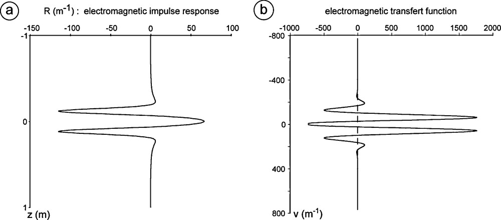
Apparent susceptibility impulse response, R(z), of a thin layer for a 0,25 m coil separation (a) and corresponding transfer function (b).
a : réponse impulsionnelle de susceptibilité magnétique apparente, R(z), d’un outil dont les centres des bobines sont écartés de 0,25 m ; b : fonction de transfert correspondante.
3.3 Deconvolution
Assuming that the demagnetizing field is negligible, which is always the case in a sedimentary context, the response of a series of layers is the direct summation of the different responses of each elementary thin layer; the problem is linear and can be solved by a Fourier transform (Desvignes et al., 1992). The measurement is expressed by the apparent susceptibility,
By taking the Fourier transform of each function, we have:
To restore the true underlying MS from the apparent MS measurements, we can use as filter, the function:
3.4 Synthetic case
With the same synthetic data corresponding to a double-cycle susceptibility variation of 0.5 m period and 500 μSI amplitude (Fig. 2a), one calculates the responses obtained by an apparatus with two coils 0.25 m apart (Fig. 2b) and with a 0.25 m long single-coil apparatus (Magnolia type, Fig. 2c). In both cases the apparent susceptibility responses are clearly different from the original susceptibility variation, both the frequency of the variations and their amplitudes are significantly altered and a direct count of the cycles would lead to a wrong result.
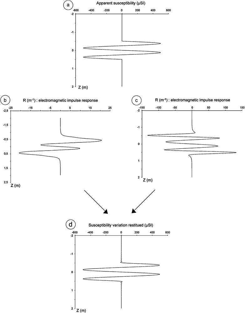
a: two-cycle susceptibility variation synthetic data; b: synthetic response of the single coil 0.25 m long apparatus; c: synthetic response of the two-coil (0.25 m apart) apparatus; d: susceptibility variation calculated for both cases by deconvolution.
a : variation synthétique de la susceptibilité présentant deux cycles ; b : réponse d’un appareil à bobine unique de 0,25 m de long ; c : réponse d’un appareil à deux bobines écartées de 0,25 m ; d : variation de la susceptibilité recalculée par déconvolution.
4 Results for the PEP1002 susceptibility log
The data were acquired in the PEP1002 borehole drilled in the Callovo-Oxfordian claystones from the floor of the ANDRA underground laboratory at a 490 m depth (Delay et al., 2006). The hole is vertical and 18.56 m long, it is cored over its entire length and just after the drilling, the whole set of cores was available for direct measurements. A correlation can also be established with surrounding boreholes especially EST103. The studied interval covers approximately the Lower Oxfordian (Thierry et al., 2006) and corresponds to dark series where some ammonites and bioturbation can be observed (Fig. 3). A series of usual logs is available: GR, electrical resistivity, density. The MS logging was performed with an apparatus with two coils 0.25 m apart, the measurement sampling step was 1 cm. The log of raw susceptibility data is presented in Fig. 3, together with the measurements carried out over the cores at a 2 cm sampling step with a MS2-E1 sensor (Bartington Ltd). Unfortunately, for technical reasons (lack of the core) a 1.5 m long gap could not be measured between 7.76 m and 9.28 m. MS measurements were also done on the EST103 borehole cores (Fig. 3), located approximately 100 m to the east of PEP1002; the measurement step was 4 cm for these cores.

Biostratigraphy and lithology for the Bure boreholes PEP1002 and EST103, and comparison of the MS records: a: MS log data PEP1002 borehole; b: MS data measured on the cores at 2 cm interval, borehole PEP1002 (5 points smoothing curve); c: MS data measured on the cores, 4 cm interval, borehole EST103 (5 points smoothing curve).
Biostratigraphie et lithologie des forages de Bure PEP1002 et EST103, et comparaison des enregistrements de la SM : a : données de SM du forage PEP1002 obtenues par diagraphie ; b : par mesure sur carottes sur le forage PEP1002 tous les 2 cm (courbe lissée sur 5 points) ; c : par mesure sur carottes sur le forage EST103 tous les 4 cm (courbe lissée sur 5 points).
At the basin scale, the correlation between MS measured on cores and logged is very good (Fig. 3). A comparison between EST103 and PEP1002 records shows the same trends and high-frequency variations. Both in raw logged data and core measurements, the dominant cycle has a 3 m wavelength defined in previous studies as eccentricity cycles (95 kyr) (Huret, 2006). On the contrary, for high-frequency variations of lower wavelengths, the amplitude looks reduced because of the instrument smoothing effect.
Time series analysis was undertaken on the PEP1002 MS data using the “Multi Taper Method” (Thomson, 1980, 1990). For each data series, the Multi Taper window was set at 2π to maximize spectral estimator resolution while maintaining suitable confidence levels. The recognition of the orbital cyclicities was obtained by the ratio frequency method (Mayer and Appel, 1999), which consists in comparing the ratio of the frequencies of two dominant cycles observed in the series to the frequency ratio of the orbital cycles fixed for the Jurassic period at between 18.2 and 21.9 kyr, 37.7 kyr and 95 kyr for respectively the precession, obliquity and eccentricity cycles (Berger and Loutre, 1994; Paillard, 2010).
Firstly, spectral analysis was made on MS core data, resampled at a 2 cm step and after removal of the linear trend. The periodogram obtained for the whole data set is presented in Fig. 4a. It looks very complex because it presents many low-frequency peaks with strong amplitude (4.1 m, 1.86 m, 1.28 m, 1.12 m, 0.97 m) close together, whereas high-frequency peaks show a very low amplitude and are not clearly expressed (0.45 m, 0.58 m). No dominant cycle can be defined. Thus, the frequency ratio of the principal periodicities does not correspond to the orbital cycle ratio. We can probably interpret the difficulty of recognizing the orbital periodicities in this spectrum by the existence of the gap (7.76 to 9.26 m). As observed by Weedon et al. (2004), some geological processes (gap/hiatuses, discontinuities, variation of sedimentation rate) create distortions in a spectrum. In this case, the effect of a gap (important in our example given the series length) generates noise around the gap, which is added to the principal cyclicities, and a decrease of the cycles amplitude. Consequently, the expression of climate cycles is affected.

Spectral analyses on PEP1002 MS data. a: spectral analysis on the MS data measured on the core, (1) et (2) analyses for 1.14 to 7.76 m and 9.28 to 18.58 intervals to minimize the (7.76 to 9.28 m) sampling gap effect; b: spectral analysis of the MS log data.
Analyse spectrale des données de susceptibilité magnétique du forage PEP1002. a : analyse spectrale de l’ensemble des données de SM mesurées sur carottes, (1) et (2), analyse réalisée sur les intervalles allant de 1,14 à 7,76 m et de 9,28 à 18,58 m pour minimiser l’effet de la lacune d’échantillonnage (de 7,76 à 9,28 m) ; b : analyse spectrale des données de SM obtenues en diagraphie.
To reduce this effect, a spectral analysis was made without considering the observation gap. Two spectra were done, the first one from 1.14 to 7.76 m and the second one from 9.28 to 18.58 m.
For the first interval, the spectrum presents three dominant cycles: 0.5 m, 1.28 m and 2.56 m. The frequency ratios of these cycles (Table 1) identify the precession (21 kyr) and eccentricity cycles (95 kyr) with 0.5 m and 2.56 m periods, respectively. The 1.28 m period seems to correspond to a harmonic of an eccentricity cycle. The second spectrum, from 9.28 to 18.58 m, expresses cyclicities similar to the first interval with precession (21 kyr) and eccentricity (95 kyr) cycles of 0.54 m and 2.5 m periods (Table 1).
Durées et rapports de durée des paramètres orbitaux calculés pour le Jurassique supérieur (Berger et Loutre, 1994) et rapports de fréquence des périodicités dominantes, observées sur les périodogrammes des intervalles allant de 1.14 à 7.76 m et de 9.28 à 18.58 m, des données de SM mesurées sur carottes du forage PEP1002.
| Orbital cycles | Precession | Obliquity | Eccentricity | P/O | P/E | O/E |
| 18.2 kyr | 37.7 kyr | 95 kyr | 0.483 | 0.191 | 0.397 | |
| 21.9 kyr | 0.581 | 0.230 | ||||
| Dominant periods | Ratio | |||||
| Intervals | a | b | c | a/b | a/c | b/c |
| 1.14–7.76 m | 0.5 | 1.28 (?) | 2.56 | 0.549 | 0.218 | 0.398 |
| 9.28–18.58 m | 0.54 | 1.02 | 2.5 | 0.549 | 0.218 | 0.408 |
A preliminary spectral analysis was made on the MS logging data (Fig. 4b) after elementary pre-processing. MS values (raw data in ppm) are expressed in μSI and show a very strong drift. It was corrected as follows:
- • elimination of a linear trend using the least-squares method. The resulting mean value was adjusted by translation to correspond to that of the core measurements (136.3 μSI);
- • maintaining the values between 2.13 m and 17.5 m to eliminate abnormally low values at the beginning of the record and to have the same value at the beginning and the end of the data series to avoid the Gibbs phenomenon.
Following these treatments, a new series (1540 points) of MS log data with a 0.01 m spacing was obtained. Spectral analysis of this new series is presented in Fig. 4b. The spectrum obtained is clearer; cycles are distinct with stronger amplitudes. Significant cyclicities of 2.92 m, 1.46 m, 0.89 m and 0.66 m periods are observed. These cycles are approximately similar to those observed with the MS core essentially for eccentricity (95 kyr) and precession (21 kyr) cycles (respectively with periodicities of 2.5/2.9 m and 0.5/0.66 m). Contrary to the MS core spectrum, the MS log spectrum shows more significant cycles (0.89 m, 1.46 m) that can be explained by a better resolution of the measurement step (0.01 m). The 1.46 m period seems to correspond to a harmonic of an eccentricity cycle. However, the MS log spectrum does not clearly show high-frequency cycles, in particular, the precession cycle (0.66 m) presents a very low amplitude. This effect is the consequence of smoothing by the apparatus, which reduces the high-frequency expressions. To minimize this effect, it is necessary to restore the underlying MS values by deconvolution. For the PEP1002 logging, the result of this restoration is presented in Fig. 5.

MS log in PEP1002: a: raw data; b: deconvoluted data.
Restitution de la susceptibilité magnétique mesurée en diagraphie dans le forage PEP1002 par déconvolution : a : courbe brute de la SM mesurée en diagraphie ; b : courbe de SM obtenue après déconvolution.
The deconvoluted MS log shows a dominant long cycle with a 3- to 4-m period observed both on the cores and the MS log raw data (Figs. 3 and 5a). For MS log data, these cycles, defined as eccentricity (95 kyr), have a better expression at the bottom of the series (10 to 18 m) than those expressed with MS data on core. The restoration of the underlying true MS values by deconvolution shows a characteristic change in the MS variations corresponding to the improvement of high-frequency variations expression. These variations with 0.5 to 1 m periods present strong amplitudes, which were not observable before processing (Fig. 5). A new spectral analysis was carried out on deconvoluted MS data. The results are presented in Fig. 6 and Table 2.
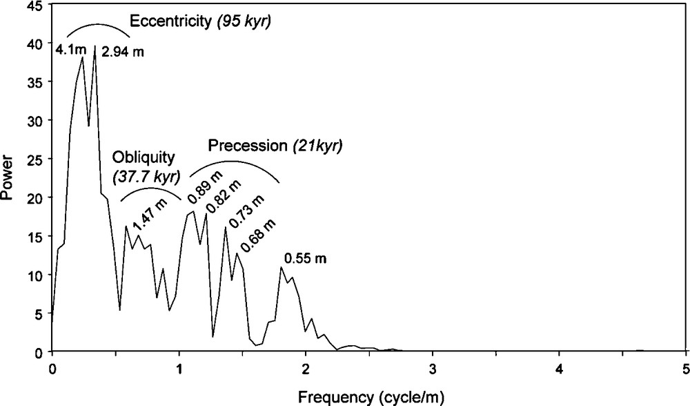
Spectral analysis obtained on the PEP1002 MS log data after deconvolution.
Analyse spectrale obtenue sur les données de SM diagraphique du forage PEP1002 après déconvolution.
Rapports de fréquence des périodes dominantes observées sur les périodogrammes des diagraphies de SM du forage PEP1002 après déconvolution.
| Orbital cycles | Precession | Obliquity | Eccentricity | P/O | P/E | O/E |
| 18.2 kyr | 37.7 kyr | 95 kyr | 0.483 | 0.191 | 0.397 | |
| 21.9 kyr | 0.581 | 0.230 | ||||
| Dominant periods | Ratio | |||||
| Intervals | a | b | c | a/b | a/c | b/c |
| Post-deconvolution | 0.55 | 1.13 | 2.94 | 0.488 | 0.187 | 0.384 |
| 0.89 | 1.72 | 4.02 | 0.517 | 0.221 | 0.418 |
For the original MS log data, the frequency ratios were used to define the periods of eccentricity (95 kyr) and precession (21 kyr) cycles, respectively at 2.92 m and 0.66 m (Table 1) in agreement with the periodicities obtained for the MS core data (Fig. 4 (1, 2)). The deconvoluted spectrum is different and presents some dominant cycles: 0.55, 0.68, 0.73, 0.82, 0.89, 1.47, 2.94 and 4.1 m (Fig. 6). Like the preceding results and with the ratio frequency analysis, eccentricity cycles are clearly expressed with 2.94 and 4.1 m periods explaining the evolution of the sedimentation rate, especially at the bottom of the series where the cycles are thicker (Fig. 5). The major difference in this spectrum is the identification of high-frequency cycles, between 0.55 m and 0.89 m periods corresponding to several peaks close together. An examination of the ratio frequencies shows an evolution of the precession (21 kyr) cycles of between 0.68 m and 0.89 m in agreement with the evolution to the short eccentricity (95 kyr) cycles (Table 2). The presence of many high-frequency periods can be interpreted as resulting from sedimentation rate changes. In Fig. 5, precession cycles have a ≈0.8 m period at the bottom of the series and a ≈0.5 m period at the top. The evolution of these cycles is not expressed in the MS core data spectrum because the resolution of the measurement step is lower; precession is represented by a large peak with an amplitude including all the periods observed in the deconvoluted spectrum. The deconvolution effect improves, and in part generates, the expression of high-frequency periods.
The deconvoluted spectrum also shows a cycle with a periodicity of 1.47 m, not expressed in the preceding spectra, that is associated by the ratio frequency study (Table 2) to the obliquity cycles (37.7 kyr).
5 Conclusion
High-resolution MS log is a light and efficient tool to record climate-forced sediment variations. Although measurements on cores or raw logging data are directly relevant as evidence of the presence of long medium-period cycles, the application of deconvolution linear filtering significantly enhances the record of high frequencies. This method improves the expression of the thin sedimentary variations usually not apparent because of smoothing effects or measurement resolution in the data. This application to well logging data is useful for examining in detail the evolution of the high frequencies and to characterize their origin, especially to detect all the climatic Milankovitch cycles and particularly the millennial-scale climate cycles of periods lower than 20 kyr unknown in the Mesozoic series. The study of their variations will give an idea of the sedimentation evolution in terms of sedimentation rate or condensation. However, these high-frequency cycles can either be harmonics of major orbital cycles or correspond to higher frequency changes. In the first case, they characterize the non-linearity of the response of the sedimentation process to orbital excitation. Their identification will allow an improvement of the knowledge of this process.
Acknowledgments
The Andra underground research laboratory organised drilling and logging operations and allowed us to use the data for cyclostratigraphic analyses. We thank the teams of Bure and Chatenay-Malabry especially Hervé Rebours, Alain Trouiller and Pascal Elion. Andra is also thanked for funding the thesis work of one of us (E.H.). We also thank two anonymous reviewers who helped us greatly improve this article.
Vous devez vous connecter pour continuer.
S'authentifier