

1 Introduction
The viscoelastic attenuation is an intrinsic property of a medium. It is due to a physical process that mainly results from the friction between the particles and fluid diffusion of the viscoelastic medium during the propagation of a seismic wave. It can be quantified through the quality factor, Q, which is the inverse of the intrinsic attenuation, or energy loss per cycle, (φ):
In the case of the strong dissipative media (e.g. Q < 30), Q is frequency-dependent and also the velocity dispersion must be considered (Červený, 2001). In our study, we assumed a weakly dissipative medium (Q > 30), with Q independent from frequency and we neglected velocity dispersion (Červený, 2001).
The velocity profile determined from real datasets recorded during the 2002 Hydratech cruise (Thomas et al., 2004) in the Storegga region (North of Norway) shows anomalies in some layers. Since the viscoelasic attenuation is an intrinsic property of a medium, it is as well as the velocity sensitive to the physical properties of the medium (e.g. Mavko and Nur, 1979; Toksöz et al., 1979), this attenuation can be used to explain the anomaly observed in the velocity profile. Several laboratory and in situ studies have shown the dependence between the viscoelastic attenuation and the nature of sediments, such as grain size and porosity (Hamilton, 1972; Mc Cann, 1969; Shumway, 1960), the presence of fluid in the sediments and its amount of saturation all affect the viscoelastic attenuation (Nur and Simmons, 1969; Toksöz et al., 1979). Nur and Simmons (1969) explain the fluid effect on viscoelastic attenuation by the relaxation time and the propagation frequency. During the passage of a high frequency wave, the fluid does not have enough time to return to its equilibrium state, therefore attenuating the wave. However, during the passage of a low frequency wave, the fluid has enough time to return to its equilibrium state, and therefore the fluid does not attenuate the wave.
Several studies have shown the effects of gas hydrates and free gas on wave viscoelastic attenuation (Gei and Carcione, 2003; Guerin and Goldberg, 2002; Matsushima, 2006; Priest et al., 2006; Rossi et al., 2007). The viscoelastic attenuation may be indicative of the presence of hydrates and free gas in the pores, and to quantify their saturation (e.g. Berryman, 1988; Gei and Carcione, 2003; Mavko and Nur, 1979; Priest et al., 2006; Rossi et al., 2007; Wyllie et al., 1962, 1963).
These considerations lead us to determine the quality factor profile in the Storegga region from real data sets acquired over the 2002 Hydratech cruise (Thomas et al., 2004).
To determine the quality factor profile with high accuracy and to obtain realistic results, we developed a long and detailed procedure based on the wave amplitude ratio in the time domain, between the main reflections observed on the recorded seismograms. To carry out our computation and to obtain the final quality factor profile, we used the ray tracing software ANRAY (Červený, 2001; Moczo et al., 1987), which we have modified to take into account the medium viscoelasticity. We name the modified software ANRAYQ.
2 Acquisition of seismic data
The 3D seismic data used for this study were acquired with a high-resolution system during the Hydratech cruise carried out by Ifremer in 2002 (Thomas et al., 2004) in the Storegga zone, North of Norway (Fig. 1). In order to produce a signal with a high frequency (central frequency at 100 Hz) and a good primary-to-bubble ratio, the seismic source was composed of one Mini-GI gun (Sodera). The amplitude of the signal source was nearly 3 bars, 1 m away from the gun.
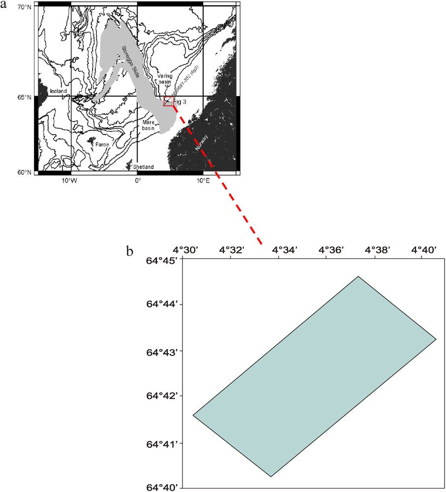
a: location of the Storegga slide area; the acquisition area is marked by the red square (http://www.hydratech.bham.ac.uk/index.htm); b: geographical position of the acquisition area (Nouzé et al., 2002).
a : localisation de la zone du glissement Storegga ; la zone d’acquisition est signalée par le carré rouge (http://www.hydratech.bham.ac.uk/index.htm) ; b : position géographique de la zone d’acquisition (Nouzé et al., 2002).
The 3D seismic data sets were acquired through the use of two 515-m-long parallel streamers, whose active length was 300 m; the distance between them was 25 m (Fig. 2). To keep noise at an acceptable level, the streamers were immersed at 3 m below the water's surface. Each contained 48 receivers (hydrophones), with a distance between two neighbouring receivers of 6 m (Fig. 2). The shooting interval was 3 s (about 6.25 m at 4.5 knots): more than a thousand shots were activated during the 3D acquisition. A thorough analysis of the recorded seismograms showed four main reflections corresponding to normal P wave reflections without conversion throughout their propagation within sediment layers (Figs. 3 and 4). We chose the shot numbers 600 and 601 for our study as these shots are located near a region of known geotechnical characteristics obtained through a past borehole study (Leynaud et al., 2007).
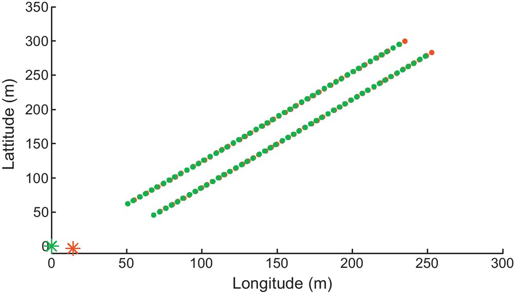
Positions of the source (asterisks) and receivers (solid circles) for the shots 600 (red color) and 601 (green color). The origin of the coordinate system corresponds to the position of the shot 601. Shots and sources coordinates were provided by Ifremer.
Positions de la source (étoiles) et des récepteurs (ronds) pour le tir 600 (rouge) et 601 (vert). L’origine du système de coordonnées correspond à la position du tir 601. Les coordonnées des sources et des récepteurs sont fournies par Ifremer.
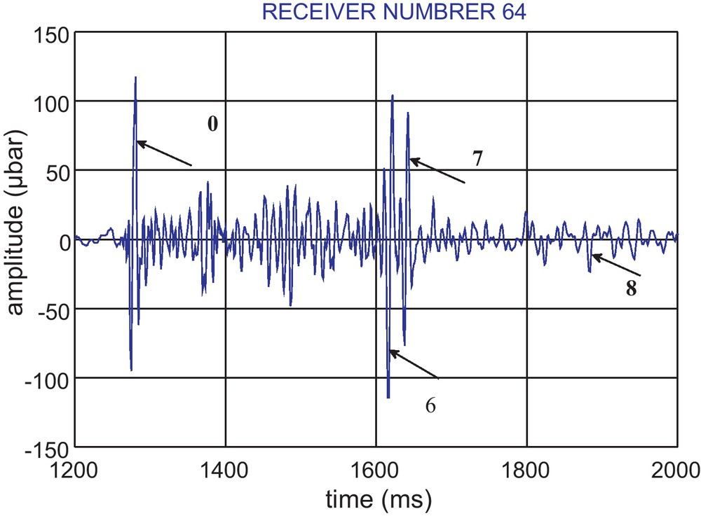
An example of the seismic data showing the response of receiver 64 to the shot 600. The main reflections (with the layers 0, 6, 7, and 8) are indicated by the arrows.
Exemple de données sismiques montrant la réponse du récepteur 64 au tir 600. Les principales réflexions (sur les couches 0, 6, 7 et 8) sont indiquées par les flèches.
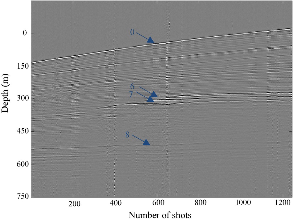
Seismic profile along the northern flank of the Storegga slide (Nouzé et al., 2002). The layers at the origin of the reflections shown in Fig. 3 are indicated by the arrows.
Profil sismique le long du flanc nord du glissement Storegga (Nouzé et al., 2002). Les couches à l’origine des réflexions montrées sur la Fig. 3 sont indiquées par des flèches.
Since no important changes are reported in the layer geometry perpendicular to the navigation direction, a 2D representation (Fig. 5) is sufficient to depict this geometry. As shown in Fig. 5, the sea bottom depth varies from 875 m to 1053 m along the profile and the sediment layers are separated by no-plane interfaces.
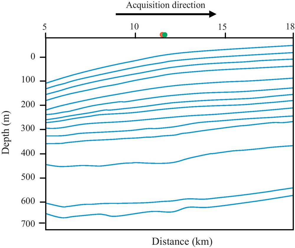
Detailed subsurface structure geometry in the plane parallel to the navigation direction (http://www.hydratech.bham.ac.uk/index.htm). The red and green points indicate the positions of shots 600 and 601, respectively.
Géométrie détaillée de la structure sub-surfacique dans le plan parallèle à la direction de la navigation (http://www.hydratech.bham.ac.uk/index.htm). Les points rouge et vert indiquent respectivement les positions des tirs 600 et 601.
The Hydratech work team of Ifremer, provided us with the geometry and the velocity profile of the structure, which were determined by using reflected data in the inversion program RAYINVR (Zelt and Smith, 1992) and Kirchhoff migration (Chavent, 1993). Also the uncertainty in velocity which equals to ±50 m/s and in depth which equals to ±5 m, were provided for us by this team.
Usually, the velocity increases with the depth (Hamilton, 1976, 1980); however the velocity profile (Fig. 6) shows a velocity decrease in layers 4, 7 and 9, respectively situated at approximately 150 m, 270 m and 550 m from the sea bottom. Note that Fig. 6 displays fewer layers than in the Fig. 5 due to blending. This is caused by similarities in the layers, parallel interfaces and equal velocities.
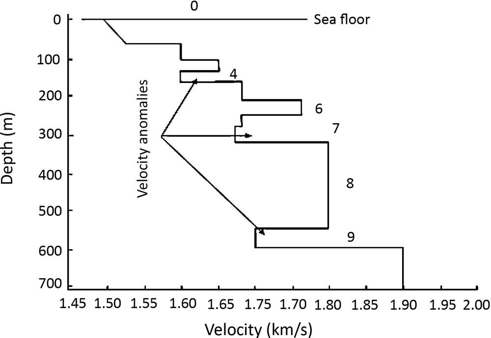
Velocity profile of the 3D acquisition area (personal communication, Ifremer), with the number of layers.
Profil de vitesse de la zone d’acquisition 3D (communication personnelle, Ifremer), avec la numérotation des couches.
3 The ANRAYQ software
The ANRAY software (version 4.01) written by Gajewski and Pšenčik (1986, 1989), is designed for ray, travel time, ray amplitude, Green's function and synthetic ray seismogram computations. Evaluations of polarization vectors, geometrical spreading and reflection/transmission coefficients are possible along the rays.
Rays can be computed by specifying the point-source location, the initial orientation of the slowness vector at the source, the location of receivers distributed along a surface, interface or vertical profile and the elastic model for each layer of the medium.
The main characteristics of ANRAY software are:
- • its ability to take into account 3D elastic, anisotropic (21 independent elastic parameters) and inhomogeneous propagation media with curved layers of nonzero thickness;
- • elastic parameters inside layers can be determined either by a vertical linear interpolation between interfaces, on which constant values of elastic parameters are specified or by a 3D interpolation by B-splines with the values of elastic parameters specified in grid points of a 3D grid;
- • ability to use a point-source situated anywhere in the medium as well as receivers distributed along the surface, interface or vertical profiles.
In order to simulate wave propagation within a 3D weakly viscoelastic medium, we replaced the real wave propagation velocity, V, by a complex velocity, V*, and we added the expression of viscoelastic attenuation factor, β, in the ANRAY software. Eqs. (1) to (3) give the expressions of V*and β:
| (1) |
The hypothesis of weak attenuation is suitable for wave propagation within a large sediment range (Lavergne, 1986). Under this assumption, the velocity dispersion is usually very small and the Q can be considered frequency-independent (Červený, 2001). Hence, Eq. (1) can be written independently from frequency:
| (2) |
| (3) |
With these modifications of the ANRAY software, the latter is able to calculate the real value of the amplitude and can be used in amplitude inversion problems. We named the modified version of the ANRAY software ANRAYQ. For more details about this modification, see Bouchaala's thesis, 2008.
4 Input parameters for ANRAYQ
To use the ANRAYQ software, we need the geometry and the geoacoustical characteristics of the medium: velocity profile and the density.
We use the velocity profile provided from the Hydratech work team (Fig. 6). Using the porosity profile acquired from the 300-m deep marine borehole (Fig. 7), the density profile can be deduced by using the relation:
| (4) |
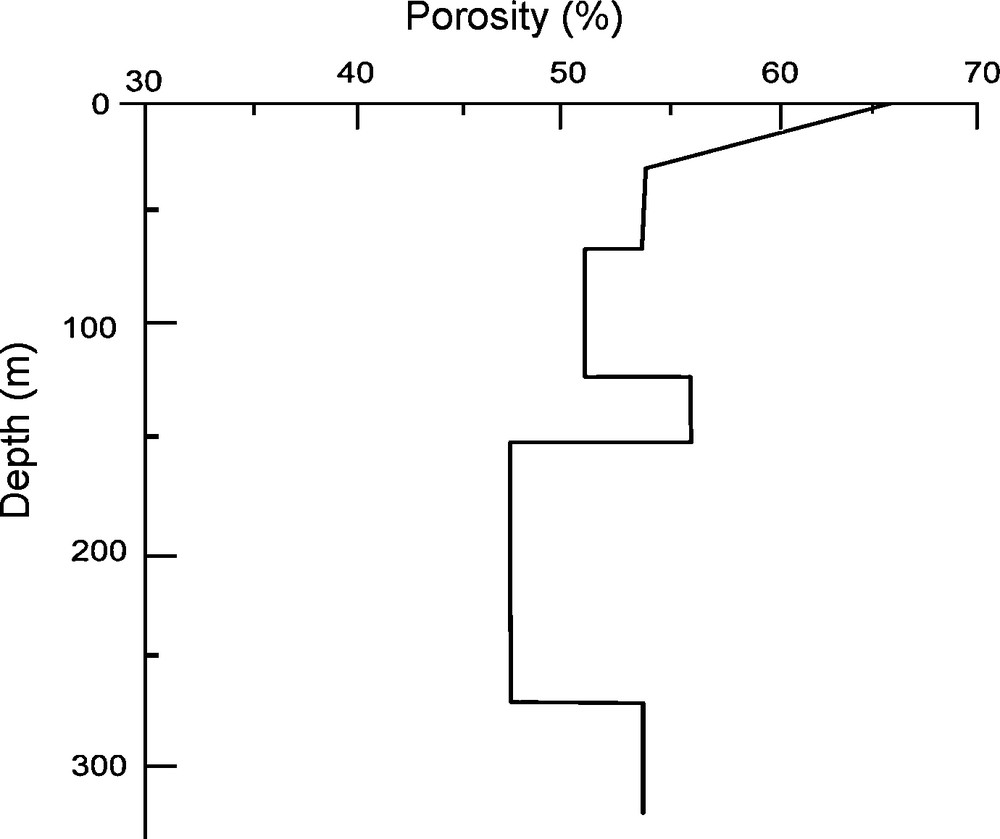
Porosity profile measured in the borehole 6404/5 (Leynaud et al., 2007).
Le profil de porosité mesuré dans le forage 6404/5 (Leynaud et al., 2007).
Since the depth of the borehole is 300 m, only the density values for sedimentary layers up to that depth are known. Empirical models (Hamilton, 1978; Wyllie et al., 1956) are used to determine the density profile for the deeper layers from velocity or porosity values. The model of Wyllie et al. (1956) allows us to relate the wave propagation velocity, V, to the porosity. According to Rider (1996), this model has been used in the determination of P wave velocity and porosity for different types of sediments (Fig. 8). Considering the soft sediments in the study region, we use the Wyllie model to calculate the theoretical density values by using curve C (Fig. 8) and Eq. (4). We then compare the theoretical values with the densities deduced from points along the known porosity profile (Fig. 9).
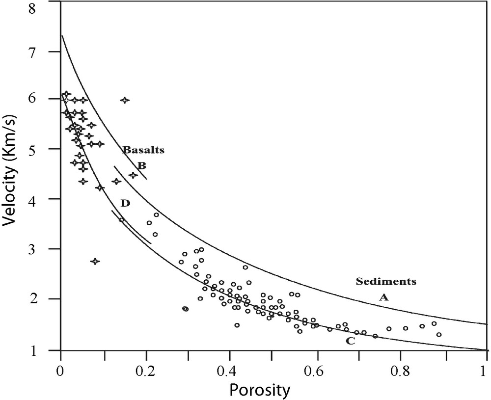
Wyllie's model curves (Rider, 1996). Curve A: compacted sediments. Curves B and D: basaltic layers. Curve C: soft sediments.
Courbes du modèle de Wyllie (Rider, 1996). Courbe A : sédiments compactés. Courbes B et D : couches basaltiques. Courbe C : sédiments mous.
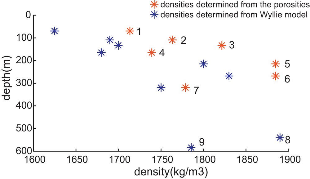
Comparison of the densities determined from the porosities measured in the borehole (red asterisks) against those issued from the Wyllie model (blue asterisks). The numbers correspond to the order of the layers in Fig. 6.
Comparaisons des densités déterminées à partir du profil de porosité mesuré dans le forage (étoiles rouges) avec celles déterminées à partir du modèle de Wyllie (étoiles bleues). Les nombres correspondent à l’ordre des couches sur la Fig. 6.
In addition to Willie's model, we tested other models, such as Hamilton's model (Hamilton, 1978). In this case, the density values calculated from Willie's model are in better agreement with the known density profile. However, there are some differences, particularly when the wave propagation velocities are between 1.5 and 1.52 km/s, as in the upper layers. When the wave propagation velocities are higher, such as in layers 6 and 7 (1.78 and 1.69 km/s, respectively), the differences between Willie's model and the known porosity profile are slight, about 3% for layer 6 and 1.4% for layer 7 (Fig. 9). Layers 8 and 9 are located below the 300-m depth-limit of the borehole, and therefore the porosity is unknown. Given the similarities in propagation velocity between layers 8 and 9 (1.81 and 1.71 km/s, respectively) and layers 6 and 7, we take the same difference values of 3% and 1.4% to calculate the deeper densities. This results in density values for layers 8 and 9 of 1896.90 and 1763.51 kg/m3, respectively. Using the approximated densities is valid due to the similarities between the layer velocities.
4.1 Density uncertainties
The mineral density is unknown, which leads to errors in the density calculation. As mentioned above, the mineral density, ρs, can vary between two extreme values, 2341 and 2770 kg/m3, which correspond to the densities ρmin and ρmax, where and . In this case (ρ = 1000ϕ + (1 − ϕ)ρs, ρs = 2420kg/m3), the maximum possible error in the density for each layer can be calculated as follows (Eq. (5)):
| (5) |
Considering the water as the only pore fluid can be not true for some layers, especially at greater depth. Other information about the fluid is required, such as concentration within the pores, nature of this fluid, temperature, etc., however it is not available in this study.
5 Method
The decreasing amplitude of a propagating wave is due to geometrical spreading, reflection/transmission and viscoelastic attenuation of the medium. The amplitude at the receiver can be expressed as follows:
| (6) |
In the case of a multi-layer medium, Eq. (6) can be expressed as:
| (7) |
We denote as the viscoelastic attenuation of the nth layer; it is equal to the ratio of the accumulated viscoelastic attenuations of the waves reflected on two interfaces, n and (n–1): . From Eq. (7), the viscoelastic attenuation of the nth layer can be expressed as:
| (8) |
Along with the reflection coefficients, the transmission coefficients are also calculated by using ANRAYQ, for the passage of the wave from the layers 1 to n-1. We use the 1D velocity profile (Fig. 6) and take account of the angular dependence and the inclination of layers for the computation of reflection/transmission coefficients.
In this study, we are able to calculate and as well as β6. We are not able to calculate because the waves reflected off the first five interfaces below the sea floor are not visible on the recorded seismograms (Fig. 3). These reflections are identified in Fig. 3, after comparison of their observed arrival times and those calculated by using the software ANRAYQ. The wave reflected from the bottom of the layer 6 and 9 are reversed (Fig. 3), because of negative impedance contrast between layer 6, 7 and 9, 10. The wave reflected from the bottom of the layer 7 is not reversed (Fig. 3) because of positive impedance contrast between layers 7 and 8.
The accumulated viscoelastic attenuation ratio, , can be expressed as:
| (9) |
| (10) |
The seismic data was preprocessed (filtering, static correction, etc.) by Ifremer, resulting in a good signal-to-noise ratio. Unfortunately, details of the preprocessing procedure, such as filtering frequencies, are not available. We determined wave amplitudes manually for the observed seismograms recorded by the 96 receivers. The amplitudes were determined to be the waveform maximum in the time domain. We consider roughly that the maximum uncertainty on the determined amplitudes, caused by manual picking, to be about 3 μbar.
In the case of a homogeneous layer, we can deduce the value of Q by using Eq. (3), from the following equation:
| (11) |
6 Results
For each receiver, we determined the average quality factor of the first six layers under the sea floor and those of layers 7 and 8. The results (Fig. 10, Table 1) show that layer 7 has the smallest quality factor values (the highest viscoelastic attenuation) and the layer 1 to 6 has the highest quality factor values (the weakest viscoelastic attenuation).
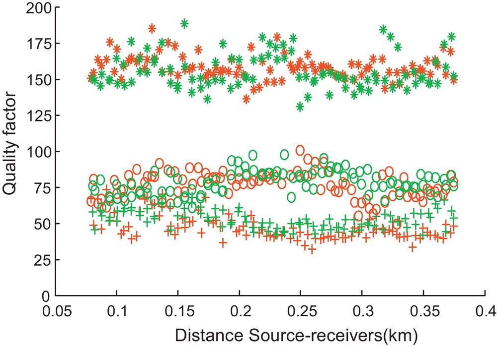
Quality factor values of the main reflections recorded by all receivers, in the case of shots 600 (red color) and 601 (green color): averaged over the layers 1 to 6 under the sea floor (asterisks); for the layer 7 (crosses), and for the layer 8 (circles).
Valeurs des facteurs de qualité des réflexions principales à tous les récepteurs, dans le cas des tirs 600 (rouge) et 601 (vert) : valeurs moyennes pour les couches 1 à 6 sous le fond de mer (étoiles), pour la couche 7 (croix), pour la couche 8 (cercles).
Valeurs moyennes du QP des 96 récepteurs pour les différentes couches, définies par l’utilisation de Eqs. (8), (10) et (11) de la section 5 (average QP), Écart-type de QP (δ). Comparaison des amplitudes calculées par le programme ANRAYQ et celles déterminées à partir de l’analyse des sismogrammes, pour les quatre réflexions principales (RMS), les valeurs de QP étant corrigées après la minimisation du RMS en utilisant l’inversion expliquée dans la section 6 et Fig. 12 (corrected QP).
| Shot 600 | Shot 601 | |||||||
| Reflection | 0 | 6 | 7 | 8 | 0 | 6 | 7 | 8 |
| Average QP | ∞ | 143 | 52.72 | 76.29 | ∞ | 141 | 46.93 | 77.12 |
| δ | 7.29 | 7.69 | 7.40 | 10.75 | 5.47 | 9.15 | ||
| RMS (μbar) | 12 | 8 | 14 | 14 | 10 | 13 | ||
| Corrected QP | 160 | 57 | 82 | 164 | 53 | 85 |
We use the averaged QP value of 96 receivers for each layer in the ANRAYQ software to recalculate the wave amplitudes. We then compared the calculated amplitudes of reflections on the sea floor and on the 6th, 7th and 8th interfaces with the mean of the amplitudes manually-picked from the observed seismograms. For example, Fig. 11 shows a shift of the calculated values from the mean of the wave amplitudes obtained from seismograms of the shot 600 and for the third reflection. The numerical estimate of this shift for all reflections and for both shots was assessed by the Root-Mean Square error, RMS (Table 1).
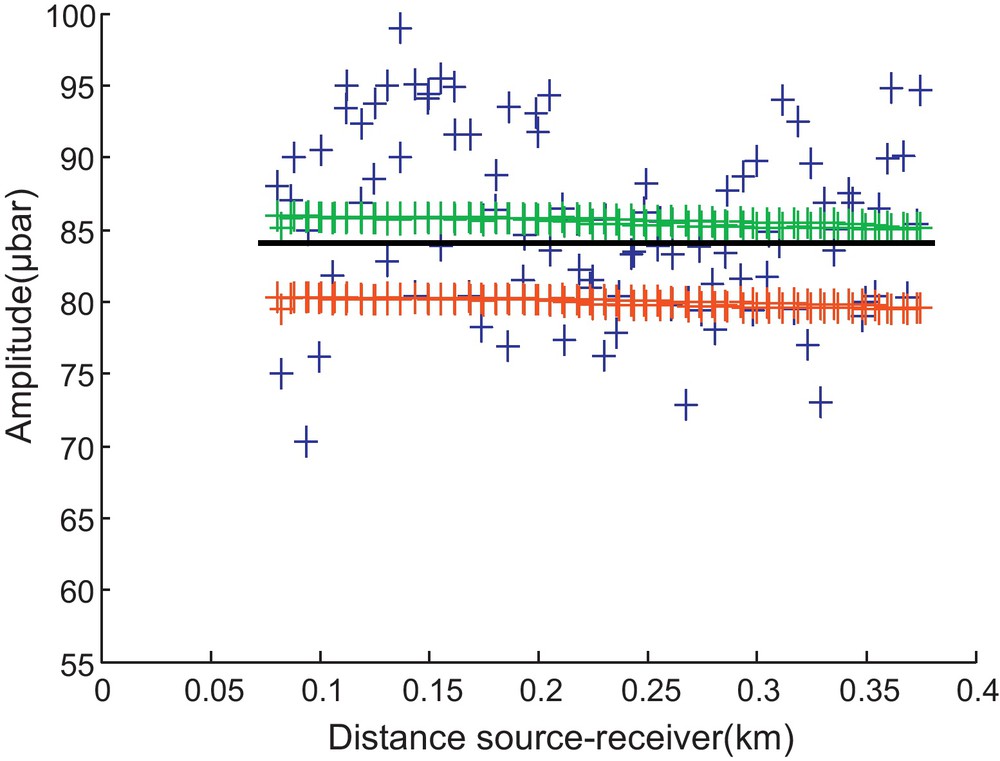
Amplitude values of third reflection for the shot 600: measured (blue crosses), calculated by the software ANRAYQ, before and after quality factor correction (red and green crosses respectively). Black solid line corresponds to the mean of amplitudes.
Valeurs des amplitudes de la troisième réflexion pour le tir 600 : mesurées (croix bleues), calculées par le programme ANRAYQ, avant et après correction du facteur de qualité (respectivement croix rouges et croix vertes). La ligne continue indique la valeur moyenne des amplitudes.
We minimize the RMS by a simple inversion, which consists of a difference calculation between the observed amplitudes and those calculated by ANRAYQ software:
| (12) |
We include the ANRAYQ software into the above algorithm. Since the initial value of the RMS is positive for each reflection, which means that Q is under estimated, we add +1 to the value of Q at each iteration. The computation is stopped when the RMS becomes less than 0.05 and relatively constant (see Fig. 12 for a further explanation of the above inversion algorithm).
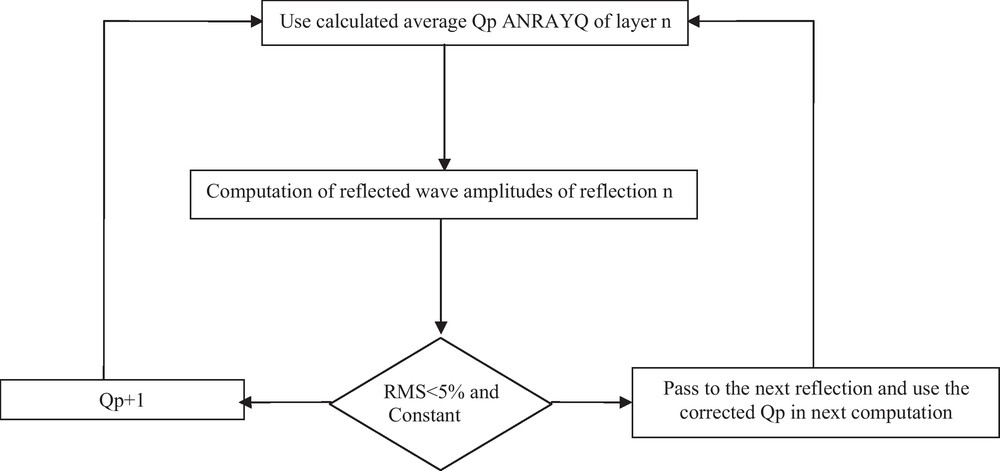
Flowchart of inversion algorithm used to correct and to improve the quality factor accuracy.
Organigramme de l’algorithme d’inversion utilisé pour la correction et l’amélioration de la précision du facteur de qualité.
The final quality factor profile (Fig. 13 and Table 1), shows that the highest average attenuation (the smallest Q value) occurs in layer 7 and the weakest average attenuation (the biggest Q value) is in the first six layers under the sea floor.
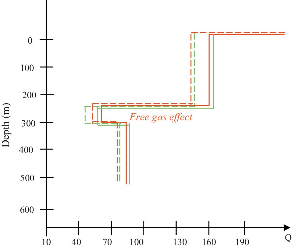
Quality factor profiles for the shots 600 (red color) and 601 (green color): quality factors determined from the ratio of the measured amplitudes (solid lines), quality factors corrected by calculation using the algorithm explained in Fig. 12 (dashed lines).
Profils du facteur de qualité pour les tirs 600 (rouge) et 601 (vert) : facteurs de qualité déterminés à partir du rapport des amplitudes mesurées (lignes continues), facteurs de qualité corrigés par calcul en utilisant l’algorithme expliqué en Fig. 12 (lignes discontinues).
7 Estimation of error in quality factor computation
As shown in the previous sections, the velocity, density and amplitude of real data determined manually are directly involved in the calculation of the quality factor. An improper determination of these parameters can cause errors in the quality factor values. In order to quantify the effect of each parameter on the calculated quality factor values, we recalculate the quality factor by adding the maximum uncertainty to an individual parameter while keeping the remaining parameters unperturbed. This test (Table 2) shows that the higher errors in quality factor values for each reflection are caused by the density uncertainty. In fact, the density is determined with less accuracy than other parameters. In addition, the quality factor of layer 8 has a maximum error. This is caused by accumulated errors from the upper layers.
Incertitudes des paramètres physiques et leurs influences sur la précision du facteur de qualité.
| Parameter | Uncertainty | Error in quality factor for each reflection | ||
| Reflection 6 | Reflection 7 | Reflection 8 | ||
| Velocity (m/s) | ±50 | ±7 | ±10 | ±10 |
| Density (kg/m3) | ±350 (1–ϕ) | ±9 | ±11 | ±15 |
| Amplitude (μbar) | ±3 | ±2 | ±3 | ±5 |
8 Discussion and conclusion
The final quality factor profile shows that the first six layers presented the lowest average viscoelastic attenuation (i.e. the highest QP), whereas layer 7 was the most attenuating layer (i.e. the lowest QP).
Finding of the highest QP from averaged QP values, relative to the first six layers, comes from water saturation due to the proximal seafloor, and hence attenuation by these layers is weak. The lowest QP value, which is found in layer 7 characterized by the lowest velocity value, can be explained by the presence of viscoelastic fluid. According to models based on Biot theory in porous media, a major cause of attenuation is wave-induced fluid flow (Carcione et al., 2010).
Fields of numerous gas chimney-type structures are observed in the seismic profile of the sedimentary structure (Nouzé et al., 2004). Therefore, the fluid contained in the layer 7 is most likely free gas and layer 6 should contain the gas hydrates. In this case, the interface which separates layers 7 and 6 can be considered as a Bottom Simulating Reflector (BSR). The free gas concentration depends strongly on the choice of saturation model (Carcione et al., 2005; Westbrook et al., 2005).
As mentioned above, there is poor resolution between the sea floor and the layer 6. Due to this complication, the quality factor of layer 6, which may contain gas hydrates, is not calculated separately from the five higher layers. The borehole carried out in the study zone (Leynaud et al., 2007) and the velocity (Hamilton, 1979; Lavergne, 1986) of the first five layers, indicate that their sediments should be composed principally from saturated sands and clays; the quality factor QP, for such sediments is between 30 and 150 (Lavergne, 1986). Since the average quality factor of the first six layers is about 160 (Table 1), the minimum value of the quality factor of layer 6 should be equal to 210.
Relatively to the layer 7, the quality factor and the velocity of layer 8 increases; however the velocity of layer 9 decreases; this indicates the existence of gas hydrates and free gas in layers 8 and 9, respectively. A comparison of the velocity ratio, VP/VS, assessed from Ocean Bottom Seismometer (OBS) data (P and S wave velocity profiles) against the value issued from Hamilton's model (1979) allowed Bünz et al. (2005), to deduce that layer 8 contains gas hydrates. The value of QP in layers 6 and 8, are in agreement with theories that assume cementation of the solid frame due to the presence of hydrate (Gei and Carcione, 2003), although there is still a debate about the effect of hydrates on seismic wave attenuation (e.g. Chand and Minshull, 2004; Guerin and Goldberg, 2002; Priest et al., 2006). On the basis of a laboratory gas hydrate resonant-column experiment, Priest et al. (2006) stated that both P and S wave attenuations are highly sensitive to small quantities of hydrate, with a peak between 3 and 5% saturation. For higher saturation, there is an attenuation decrease. Priest et al. (2006) explained the decrease of attenuation by the cementation of grain contacts caused by increasing hydrate concentration, which leads to an encasement of the sand grain and an infilling of the pore space. As the sand grains become encased, the potential for squirt flow into the pore space is reduced. Therefore, according to these studies we can deduce that the concentration of gas hydrates in layer 6 and 8 should be higher than 5% and we can consider weak hydrates dissociation to free gas.
The comparison of QP and P wave velocity profiles highlighted a good agreement between the variations of velocity and QP values; indeed, the lowest values were found in the free gas-containing layer. The upper interface of the fourth layer cannot be considered as a BSR, because the conditions required for gas hydrate formation (pressure and temperature) are not satisfied at this depth (Gei and Carcione, 2003). The velocity anomaly at this layer can be explained by an overpressure of the water trapped in this layer.
Shortage of time prevented us from determining the quality factor from all shots, but since the structure layers were considered homogeneous and their lithology was assumed as space-independent, the quality factor can be considered to slightly vary within each layer. Hence, the quality factor calculated for each layer can be considered as representative.
Acknowledgements
We thank Yannick Thomas and Hervé Nouzé for the real data and their explanations about these data; we also thank Catrina Alexandrakis and Rosi Davi for their linguistic help.