

1 Introduction
The ground-penetrating radar reflection (GPR) technique, a geophysical method based on high frequency (10–2300 MHz) electromagnetic (EM) wave propagation, can provide very detailed and continuous images of the subsurface. One of the goals of GPR measurements is to determine the geometries of fine structures by imaging the shallow subsurface. In general, the GPR measurements are performed on nearly flat surfaces and in this case, if highly dipping reflections and/or diffractions are present in the data, a standard migration is needed in order to precisely determine the geometries of shallow structures (Feng et al., 2009; Zeng et al., 2004).
For a variable topographic relief, a standard processing procedure includes the application of static shifts (Annan, 1991; Sheriff and Geldart, 1995) followed by a classical migration commonly performed with a flat datum plane. Nevertheless, this processing technique does not give good results for large topographic variations. In addition, the inadequacy of conventional elevation static corrections to take into consideration a gentle to rugged topographic relief was shown to be a particular problem (Lehmann and Green, 2000). To obtain reliable images from GPR data acquired on areas showing irregular topography, a special processing that takes topography into account may be required. Although the relief variation, in seismic acquisition, is small compared to the investigation depth, various migration methods with topography have been developed for seismic data (Berryhill, 1979; Bevc, 1997; Shtivelman and Canning, 1988; Wiggins, 1984). These migration techniques could be of a more important use in GPR data than in seismic, as the target structures have often the same order of depth as the topographic relief variations.
Lehmann and Green (2000) adapted a topographic migration for GPR data based on the Kirchhoff algorithm proposed by Wiggins (1984) for the seismic data collected in mountainous areas. According to these authors, the topographic migration should be considered when the surface slope exceeds 10%. This migration method has been successfully used, in 3D, by McClymont et al. (2008) for the GPR data acquired on active fault areas showing a rugged topography.
In this article, we first present an overview of Kirchhoff's topographic migration algorithm and demonstrate the diffraction equation used in this method as presented by Lehmann et al. (1998). To show the efficiency of the method, we first use synthetic data from a single diffraction point model, and compare the migration results with flat datum and topography, respectively. Then, we present two different examples of real GPR data recorded in areas presenting local and large topographic variations as well as a mean slope of less than 10%. The first example is from a dry sand dune of the Chadian desert, presenting a high velocity medium with local topographic variations, while the second one is from Mongolia, presenting a topographic slope of 10%. Finally, we show and compare the results of GPR profiles processed with static shift followed by migration, migration followed by static shift and topographic migration, and discuss the superiority of the later one even in the cases where the topographic slope is lower than 10%.
2 The Kirchhoff topographic migration
2.1 The Kirchhoff migration
Let us consider a simple 2D geological model (x–z plane) composed of a diffraction point (diffractor) placed on a perfectly resistive medium with a constant EM velocity. The coordinates of this diffractor are xd and zd, respectively (Fig. 1a). We assume a zero-offset survey with transmitting and receiving antennas that move on a flat horizontal surface at z = 0 (dashed line in Fig. 1a). In this case, the result of the zero-offset GPR profile in time (x–t plane) will be a diffraction hyperbola (shown by the dashed line in Fig. 1b) and the electric field variation can be described by a scalar wave propagation equation, which is similar to the acoustic wave equation (Leparoux et al., 2001).
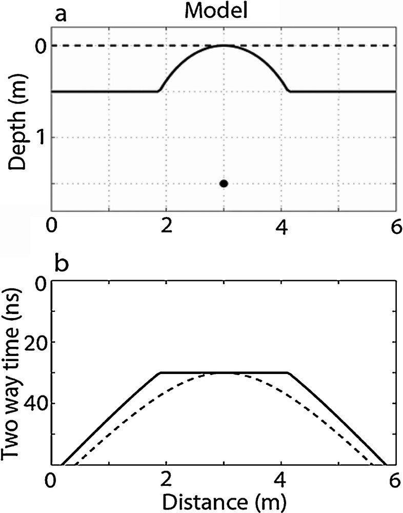
a) Geological model composed of a diffraction point (black dot) placed on (xd, zd). The dashed line represents the flat datum plane located at z0 = 0, while the thick one shows the acquisition surface with topography; b) zero-offset ground-penetrating radar profiles obtained by moving the antennas on both surfaces. The dashed line (a diffraction hyperbola) corresponds to the acquisition on the flat datum plane (dashed line in Fig. 1a), while the thick line represents the case where the acquisition is performed on the surface with topography (thick line in Fig. 1a). Note the difference between the two observed curves.
a) Modèle géologique composé d’un point diffractant (point noir), placé en (xd, zd). La ligne pointillée représente la surface plane théorique, située en z0 = 0. La ligne épaisse représente la surface d’acquisition réelle. b) profil géoradar à offset nul, obtenu en déplaçant les antennes sur les deux surfaces. La ligne pointillée (hyperbole de diffraction) correspond à l’acquisition sur la surface plane théorique (ligne pointillée, Fig. 1a). La ligne épaisse représente l’acquisition sur la surface avec topographie (ligne épaisse, Fig. 1a). Noter la différence entre les deux résultats.
The goal of the migration is to find the geological model (in the x–z plane) from the zero-offset GPR profile (in the x–t plane). For a resistive medium (high-frequency approximation), we can use Kirchhoff's method that gives the wave field at the location of the diffractor (xd, zd) from the zero-offset wave field measured at the surface z = 0 (Feng et al., 2009; Schneider, 1978). Practically, the Kirchhoff migration will calculate the diffraction hyperbola (migration template) for each point of the GPR profile and, by adding the amplitudes along the template, will place it at the top of the template in the migrated profile (Claerbout, 1985; Yilmaz, 2001). Migrating each of these points for a given velocity will focus the amplitudes at their correct positions and the reflector is imaged with its true position and dip angle.
2.2 Effect of the topography
When GPR measurements are performed over a surface with topography, the migration template is no longer a diffraction hyperbola; instead, it will be a distorted diffraction curve. This is shown in Fig. 1 where the topography is chosen to be a circle whose centre is on the diffraction point (xd, zd), and on both sides of which the topography is flat (see the thick line in Fig. 1a). The distance between the diffraction point and the antennas (in zero offset), moving on the surface along the circle, is constant. Therefore, the migration template, shown by the thick line in Fig. 1b, will be flat on the top, and on both sides it will be represented by two flanks of a diffraction hyperbola. In this case, the imaging result of the classical Kirchhoff migration with a flat datum plane will be spurious (Fig. 4). For this reason, we absolutely need to take into account the topography of the GPR acquisition surface.
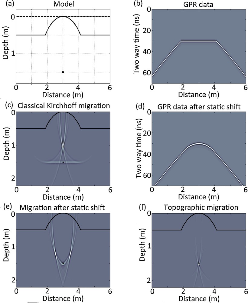
a) Diffraction point model, with topography (thick line); b) zero-offset ground-penetrating radar data corresponding to a survey over this area. Note the distorted diffraction curve (migration template); c) classical Kirchhoff migration with a flat surface at z = 0; d) GPR data after the static shift, e) classical Kirchhoff migration after static shift; f) The result of the topographic migration; the thick line on Fig. c, e and f corresponds to the real topography.
a) Modèle du point diffractant avec la topographie (ligne noire continue) ; b) données géoradar à offset nul correspondant à un levé sur la zone. À noter : la distorsion de la courbe de diffraction (maquette de migration) ; c) migration de Kirchhoff classique avec une surface plane à z = 0 ; d) données géoradar après corrections statiques ; e) migration de Kirchhoff classique après corrections statiques ; f) migration avec topographie. La ligne noire continue en c, e et f correspond à la vraie topographie.
2.3 Migration with topography
For the standard Kirchhoff migration, at a location x on the surface z = 0 (i.e. the antennas move on the flat datum plane), the two-way travel time t(x) along the grey line path in Fig. 2 is given by:
| (1) |
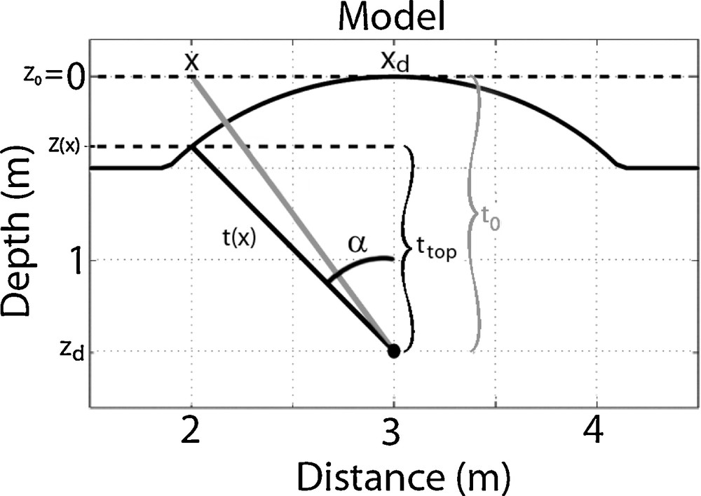
Schematic presentation showing the topographic correction for the Kirchhoff migration. For a given position x at the surface z0 = 0, we take into account the topography z(x) instead of considering the flat datum plane (dashed line at z0 = 0). The travel time t(x) is now calculated along the thick line path rather than along the grey line one.
Schéma illustrant la correction topographique pour la migration de Kirchhoff. Pour une position x donnée sur la surface z0 = 0, la topographie z(x) est utilisée au lieu de considérer la surface plane théorique (ligne pointillée à z0 = 0). Le temps de trajet t(x) est alors calculé le long de la ligne noire plutôt que de la ligne grise.
Correcting for the topography means to choose for the migration template the thick line of Fig. 1b, instead of using the dashed one, which is exactly a diffraction hyperbola. This will allow the template to follow exactly the real travel path of the GPR data. Indeed, for the same x location (Fig. 2), the z position of the antennas (moving on the rugged surface) has been changed and the two-way travel time t(x) is now calculated along the thick line path in Fig. 2 to obtain:
| (2) |
with:
| (3) |
| (4) |
This equation is the same as the one given without any demonstration by Lehmann et al. (1998) in the case of a 2D migration. Fig. 3 presents an overview of the different steps to compute the topographic migration. We have used the same notations as in equations (1) to (4).
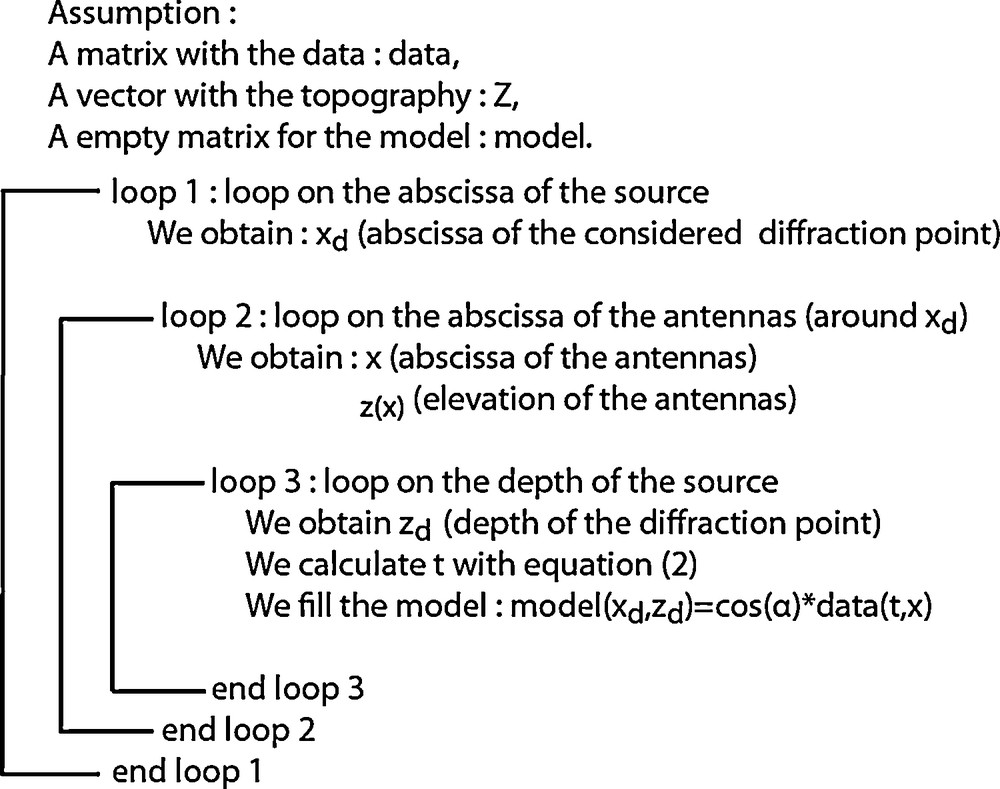
Diagram showing the different steps of the Kirchhoff topographic algorithm. The names of the variables are the same as the ones used in equations (1) to (4) and Fig. 2. A first matrix with the data (data), a vector Z with the topography, and an empty matrix for the model (model) are required. The algorithm starts with a first loop on the x position of the diffraction point (xd). We move around the xd position to get x and z(x) (position of the antenna) in a second loop. The third loop is running on the depth location of the diffraction point (zd). Finally, we calculate the two-way travel time between the antennas location (x, z(x)) and the diffraction location (xd, zd) using equation (2) to fill the model.
Schéma représentant les différentes étapes de l’algorithme de la migration de Kirchhoff. Les noms des variables sont les mêmes que ceux utilisés dans les équations (1) à (4) et la Fig. 2. Une première matrice avec les données (data), un vecteur Z comprenant la topographie, et une matrice vide pour le modèle (model) sont requis. L’algorithme commence par une première boucle sur l’abscisse du point diffractant (xd). Dans une seconde boucle, la position des antennes est déplacée autour de la position xd pour obtenir x et z(x) (position des antennes). La troisième boucle incrémente sur la profondeur du point diffractant considéré (zd). Le temps de trajet aller-retour entre la position des antennes (x, z(x)) et la position du point diffractant (xd, zd) est calculé via l’équation (2) pour remplir la matrice modèle (model).
In Fig. 4 we compare the results of the classical migration with flat datum plane, the classical migration after static shift and the topographic Kirchhoff migration. Fig. 4b displays the synthetic radargram computed with the model of Fig. 4a. This radargram is obtained by using a second order Ricker source having a dominant frequency of 500 MHz, located over a homogeneous medium with a velocity of 0.1 m/ns. The distance between traces is 2 cm.
Fig. 4c shows the classical migration of the zero-offset GPR synthetic data of Fig. 4b. One can see a flat horizontal 2-m-wide layer located at a depth of 1.5 m, as well as a bright spot in the middle of the section at a depth of around 1 m (Fig. 4c). The imaging result is very poor and might lead to a misinterpretation of the data. The actual classical procedure is a static shift followed by a classical migration. Fig. 4d shows the synthetic data after the static shift, and Fig. 4e displays the migration after the static shift. The result seems to be better than the one of Fig. 4c. In Fig. 4e we observe not only a bright spot at the correct depth of 1.5 m, but also two strong spots located on both sides of the diffraction point (around a depth of 1.2 m). In Fig. 4f, we present the result of the topographic migration appropriately weighted by an amplitude factor proportional to cos(α) = ttop/t(x) which also depends on the topography (Fig. 2). The amplitude factor is added to take into account the directivity factor that describes the angle dependence of amplitudes and is given by the cosine of the angle between the propagation direction and the vertical axis (Claerbout, 1985; Yilmaz, 2001). The data are well imaged and, as expected, are focused on a single bright spot located at its real depth of 1.5 m (Fig. 4f).
3 Real ground-penetrating radar data examples
3.1 The Chad Dunes
The first example is a GPR profile collected over an aeolian dry dune in the Chadian desert (Bano et al., 1999). The goal of this survey was to image the interior and the base of the dunes to better understand sedimentological processes. The GPR profile has been obtained using a 450-MHz shielded antenna. The acquisition mode was a constant offset of 0.25 m, the antennas were moved by 0.125 m steps with a stack of 64 to improve the signal-to-noise ratio.
A standard processing (with in-house interactive GPR software) has been applied and the resulting profile is displayed in Fig. 5a. The following processing sequence was used: constant shift to adjust the time zero followed by normal move-out corrections; running average (DC) filter to remove the low frequency; flat reflections filter to remove some clutter noise (continuous flat reflections) caused by multiple reflections between shielded antennas and the ground surface; a band-pass filter and finally a time-varying gain function. The same standard processing is applied to all GPR data presented in this section.
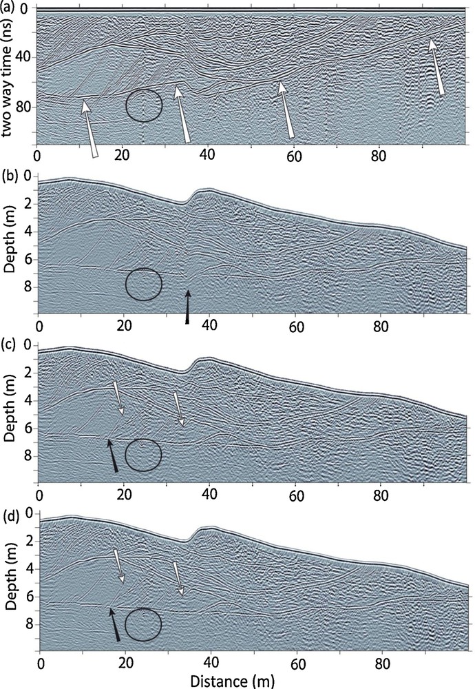
Ground-penetrating radar profile acquired over a Chadian dry dune with a 450-MHz antenna. a) After the standard processing described in the text. b) after a standard migration followed by a static shift, with a velocity of 0.18 m/ns. This same velocity has been used for all following migrations and topographic corrections; c) after static shift followed by standard migration and d) after Kirchhoff's topographic migration.
Profil géoradar enregistré sur une dune de sable sec, dans le désert du Tchad, avec une antenne de 450 MHz. a) Après le traitement classique décrit dans le texte ; b) après migration classique suivie d’une correction statique, avec une vitesse de 0,18 m/ns. Cette vitesse a été utilisée pour toutes les migrations et les corrections statiques qui suivent ; c) après corrections statiques, suivies par une migration classique ; d) après migration topographique de Kirchhoff.
The GPR profile of Fig. 5a shows complex geometries, with imbricate reflections corresponding to different deposit phases. The undulating reflection indicated by four white arrows in this figure represents the base of the dune, which in fact is nearly flat and consists of pebbles (> 2.0 mm in diameter). This reflection stems from the contact between the aeolian sands near the surface and deeper lake deposits consisting of an unconsolidated silty sandstone layer of very fine to medium grain size. In order to apply the topographic static shift and/or migration, we need to know the velocity of the GPR waves. In Fig. 5a, we also observe a nice 10-m-wide (80 traces) diffraction hyperbola situated just under the base of the dune (see black circle). After analyzing this diffraction, with different velocities, we found that it can be fitted very well with a constant velocity model of 0.18 m/ns. This value represents an average velocity from the surface of the dune to the diffraction point and it is in good agreement with values found in the literature for dry sands (Gómez-Ortiz et al., 2009; Guillemoteau et al., 2012).
Fig. 5b shows the same GPR profile as in Fig. 5a, but when a standard migration followed by topographic corrections is performed, using a velocity of 0.18 m/ns. The topography shows a local variation of about 30% (at profile coordinate 38 m, black arrow in Fig. 5b) and its global variation of about 5 m (5%) is comparable to the investigation depth. The diffraction hyperbola is well collapsed (at profile coordinate 25 m, black circle) and the reflection from the base of the dune is roughly flattened. Below the area of high topographic gradient (38 m horizontally), we observe a very bad feature (black arrow). The whole area looks blurred, and reflectors are losing consistency. The results of the standard migration followed by topographic corrections are bad.
Fig. 5c presents the profile after a static shift followed by a standard migration. The migration hyperbola (black circle) is slightly over-migrated. The bad feature indicated by the black arrow in Fig. 5b is corrected. The reflectors are now consistent and the dipping reflector shown by the black arrow (Fig. 5c) has been moved up-dip.
Fig. 5d presents the topographic migration with the same velocity (0.18 m/ns, as in both previous cases) and a specific migration template 13 m wide (100 traces) has been chosen, which is slightly larger than the width of the observed hyperbola (10 m) on the profile. The base of the dune is flattened and the diffraction at 25 m is now correctly focused on a single point inside the black circle, which justifies our choice of 0.18 m/ns for the GPR velocity. The dipping reflector shown by the black arrow has undergone a vertical and horizontal shift of 1.1 and 3.8 m, respectively. It starts at the base of the dune and goes up-dip rightwards as expected (on the non-migrated section of Fig. 5a, these reflections were crossing the base of the dune).
The measured dips on the topographic migrated section of the same reflectors (shown by white arrows) are slightly larger than the dips measured in Fig. 5c (static shift followed by standard migration). Their values are now 26.5° and 19.5° on the topographic migrated section, instead of 25° and 17.7° in Fig. 5c. Although the global topographic variation of the profile does not exceed 5%, the result of the topographic migration is slightly better than the result of the static shift followed by the standard migration. Remember here that the later routine over-migrates the data at large depth (case of the diffraction under the base of the dune).
Fig. 6 shows a portion of the profile of Fig. 5d with topographic migration for different velocities ranging from 0.16 m/ns (left) to 0.20 m/ns (right) with a 0.1 m/ns increment. The hyperbola is not collapsed for the two first figures, while it is over-migrated for the last two ones. The middle figure shows the migrated image with the correct velocity of 0.18 m/ns. The depths and the dips of the reflectors are also changed. The depth of the diffracting point is ranging from 6.5 m (for a velocity of 0.16 m/ns) to 7.8 m (for a velocity of 0.20 m/ns). Therefore, a change of around 5% in the velocity causes a change in depth of nearly 0.3 m (for a depth of around 7 m). The dip of the reflector indicated by the arrow is ranging from 22.6° (velocity of 0.16 m/ns) to 29.9° (velocity of 0.20 m/ns). The dip increases by roughly 2° per 0.01 m/ns velocity increase. To have a correct migration, we conclude that the precision in the estimation of the velocity should be better than 5% of the true velocity.
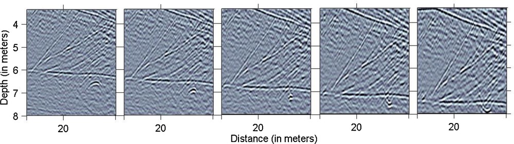
Detailed area of the base of the dune showing the topographic migration of the diffraction curve (under the base of the dune) for different velocities ranging from 0.16 m/ns (on the left) to 0.20 m/ns (on the right) with a 0.01 m/ns increment. The figure in the middle shows the correct topographic migration with V = 0.18 m/ns.
Zoom sur la base de la dune, montrant la migration topographique de l’hyperbole de diffraction (sous la base de la dune) pour différentes vitesses allant de 0,16 m/ns (à gauche) à 0,2 m/ns (à droite), avec un incrément de 0,01 m/ns. La figure du milieu montre la migration topographique correcte avec une vitesse de 0,18 m/ns.
3.2 Example of a fault in Mongolia
In 2010, we conducted a GPR campaign in Mongolia, 80 km to the west of the capital Ulaanbaatar. The context of this study was seismic hazard. Fig. 7 shows a GPR profile obtained with an unshielded 50 MHz Rough Terrain Antenna (RTA). The profile is more than 200 m long and is perpendicular to the Hustay Fault. This is in a context of a very low slip rate (most likely less than 1 mm per year), and the fault geomorphology has been smoothed during a long period of erosion. Therefore displacements in the topography are not observable. However, in the field, evidences of the fault plane are still visible. Most of the profiles acquired in this area display a strong reflection, which corresponds to the fault plane. These profiles give complementary information such as the dip of the structure and the exact location of the fault near the surface to help design the layout of future palaeoseismic campaigns. The acquisition mode was a constant offset of 4.1 m; traces have been recorded every 0.2 m with a stack of 16 to improve signal-to-noise ratio.
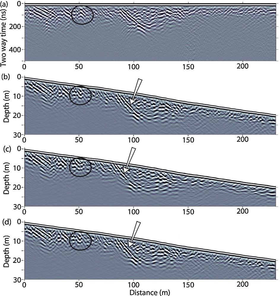
Ground-penetrating radar profile obtained in Mongolia with an unshielded 50 MHz Rough Terrain Antenna. a) Standard processing (see the text); b: with standard migration followed by static shift; c) with static shift followed by standard migration and d) with topographic migration. Static corrections and migration are performed with a constant 0.12 m/ns velocity.
Profil géoradar obtenu en Mongolie avec une antenne non blindée de 50 MHz. a) Après traitement standard des données (voir dans le texte) ; b) après migration standard suivie par une correction statique ; c) après correction statique suivie par une migration classique et d) après migration topographique. Les corrections statiques et les migrations ont été faites avec une vitesse constante de 0,12 m/ns.
The processing used to obtain Fig. 7a is similar to the one used in the case of the Chadian GPR data. A velocity analysis, which is not presented here, has been done over the surveying area by analysing diffraction hyperbolae present in the GPR data. A mean velocity of 0.12 m/ns has been determined for the whole area. As in the previous example, the topographic variation of 20 m (slope less than 10%) is comparable to the investigation depth. Figs. 7b, c and d respectively display the data after standard migration followed by static shift, static shift followed by standard migration, and topographic migration. The diffraction hyperbola indicated by the black circle is well focused in Fig. 7b and d, and appears slightly over-migrated in Fig. 7c (as in the case of the Chad dune). The dipping reflector (fault plane) indicated by the white arrow now displays a constant slope down to a depth of 24 m in Fig. 7b and d. However, on the section of Fig. 7c, the reflector is attenuated at a depth of 17 m and has lost its continuity. Its dip angle is changing from 32.2° (migration and static shift) to 34° (static shift and migration and migration with topography). The main observation is the location of the reflector, which is very similar in the cases of Fig. 7b and d, while in Fig. 7c the reflector has been shifted (5.5 m horizontally and 2.6 m vertically) and is reaching the surface. In this case, the migration followed by static shift seems to give more convincing results than the static shift followed by migration (which is the opposite of what was observed in the Chadian dune example). From this result, we conclude that topographic migration should be considered at any location where the subsurface shows steep dip angle structures (exceeding 30°), even in the case where the surface slope is less than 10%.
As in the previous case, we performed a velocity sensitivity analysis by using a topographic migration of the fault plane reflection with different velocities ranging from 0.1 m/ns to 0.14 m/ns with a 0.01 m/ns step. After topographic migrations, the slope of this reflector is varying from 28.9° to 39.5° and increases by roughly 2.65° for a 0.01-m/ns increase in the velocity. In this case, for a correct topographic migration, the estimation of the velocity should be better than 8%.
4 Conclusion
In the presence of relief variations of the same order as the investigation depth of GPR data, a topographic migration is necessary to correctly locate the dipping reflectors and focus the diffractions. The topographic migration presented in this article is based on Kirchhoff's algorithm similar to the method proposed by Lehmann and Green (2000). The application may be more useful for GPR data than for seismic data, as the topographic variations are comparable to the depth of the target structures. We demonstrate the template migration equation, as a function of the topography, along which the amplitudes are added together to give a single point on the migrated section.
By comparing processed sections obtained from GPR data measured over media of high EM velocity (dry sand) having large local topographic variations within a global topographic slope of 5%, we show that reflectors obtained by standard processing (static shift corrections followed by migration) have dip angles that deviate from the angles in a topographically migrated profile by 1 to 2 degrees. Their locations are also changing by a few meters, even for reflectors close to the surface. Thus, for high velocity media with large local topographic variations, even in the case where the global surface slope does not exceed 5%, the application of the topographic migration is necessary and efficient. We also show that topographic migration should be considered at any location where the subsurface shows steeply dipping structures (> 30°), even for surface topographic slopes of less than 10%. Finally, we have shown that the precision in the velocity estimation should be from 5 to 10% of the true velocity, in order to have a correct topographic migration.
Acknowledgement
We thank the reviewers of the initial draft of this article, C. Çağlar Yalciner, S. Garambois, and F. Rejiba for their help in improving the manuscript.