

1 Introduction
Reservoir properties are controlled primarily by the sedimentary architecture and facies association distribution, but are strongly modified during early to late diagenetic history. Understanding and predicting the spatial distribution of reservoir heterogeneities induced by diagenesis is thus a crucial question to tackle in reservoir characterization and modeling (Ehrenberg and Nadeau, 2005; Lucia, 1999; Moore, 2001).
This is particularly true for carbonate reservoirs, as carbonates present a strong chemical reactivity to acid/base systems and can be affected by a large diversity of reactions, such as dissolution, precipitation or recrystallization (Ehrenberg et al., 2006; Lucia, 1999; Qing Sun and Esteban, 1994). Thus, one key point for carbonate reservoir modeling is to integrate quantitatively the diagenetic overprint into the sedimentary model. However, joint geostatistical simulation of facies and associated diagenesis have only recently been investigated (Barbier et al., 2012; Doligez et al., 2011; Labourdette, 2007; Pontiggia et al., 2010).
This paper proposes a complete workflow from data acquisition to geostatistical modeling of both facies and diagenesis (bi-plurigaussian methods), and its application to an outcrop analog, the Early Eocene Alveolina Limestone Fm. of the Graus–Tremp Basin (NE Spain). The workflow includes a sedimentological characterization (depositional environments and sedimentary architectures), and a detailed description of the diagenesis that affected these series. These results were used to define a modeling workflow, which integrates both the sedimentological and diagenetic constraints in a stochastic simulation.
2 Geological setting
The study area (named Serraduy) is located in the Graus–Tremp Basin (Huesca Province), on the southern flank of the Spanish Pyrenees (Fig. 1). This basin corresponds to the easternmost part of the South Central Pyrenean unit, made up of several units (Boixols, Montsec, Sierras Marginales; López-Blanco et al., 2003), detached at a Triassic décollement level and transported southward (Fig. 1). The Graus–Tremp Basin is therefore considered as a piggyback basin of Eocene age, filled and progressively carried southward over the low-angle Montsec thrust. In terms of paleogeography, the Graus–Tremp Basin was characterized during Paleocene–Eocene times by an elongated gulf connected westward to the Bay of Biscay, located at the southern border of the Pyrenees axial zone, at a tropical paleolatitude (Hay et al., 1999).
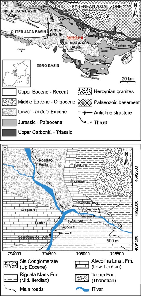
(Color online.) A. Geological map of the south central Pyrenees (modified from Vincent, 2001) and location of the study area (Serraduy). B. Geological maps showing the main lithostratigraphic formations of Early Eocene age in the Serraduy area, with location of the sedimentary sections described in this study (UTM coordinates, WGS84).
The studied Alveolina Limestone Fm. (Lower Eocene, Ilerdian stage, 56–57 Ma) is part of the Early Tertiary basin fill. This formation is onlapping from the south onto the Late Paleocene continental Garumnian Fm. (Fonnesu, 1984), and corresponds to a renewed marine incursion in the South Pyrenean Gulf at the transition between Paleocene and Eocene.
3 Sedimentological characterization
3.1 Facies associations, sedimentary architectures and depositional environments
In the study area, ten sedimentary sections were logged (Fig. 1). From these sedimentary sections, sixteen facies were defined by texture, sediment constituents, sedimentary structures, fossils and/or trace fossils (Hamon et al., 2012; Rasser et al., 2005; Scheibner et al., 2007). These facies were grouped in ten facies associations (named F1 to F10) corresponding to ten depositional environments. The latter will be used as inputs for modeling purposes, and will be referred as sedimentary lithotypes (standard terminology for sedimentary input in modeling workflow). The sedimentary architecture was also directly assessed on the field by following the main discontinuities (erosional surfaces, hardgrounds) and interpreting photo-panels with line drawings. A 3D geological model illustrating the general architecture and the sedimentary lithotype distribution of the Serraduy area is proposed in Fig. 2.
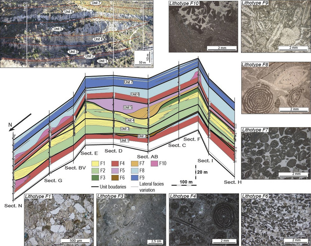
(Color online.) 3D Model illustrating the general architecture, modeling units and depositional environments (sedimentary lithotypes) distribution of the Ilerdian Alveolina Limestone Fm. in the Serraduy area. F1: Siliciclastic channels and lobes; F2: Shaly lobe fringe; F3: Interdistributary restricted pond; F4: Beach/Inner-ramp; F5: Lagoon; F6: Tidal channel; F7: Tidal megadune; F8: Mid-ramp; F9: Outer ramp; F10: Bioconstruction.
The first unit (unit 1) is composed of three lithotypes (F4, F8 and F10). At the scale of the studied area, the base of the series (unit 1) is dominated by a homogeneous facies: an Alveolina and Orbitolites dominated wackestone to packstone, with a low to medium fragmentation, and common Lucina in living position (F4 – Fig. 2). In the southern part of the area, this unit passes laterally to a Nummulites and Operculina wackestone, moderately bioturbated, without any sedimentary structure (F8 – Fig. 2). The high abundance of Orbitolites observed in F4 suggests a very proximal setting such as a beach, or inner-ramp environment (Geel, 2000). It passes southward to a mid-ramp setting, as attested by occurrence of Nummulites and Operculina (F8; Geel, 2000; Rasser et al., 2005). On the northern part of the area, a coral-dominated bioconstruction (averaging one hundred meters of lateral extent and 12 meters in height) is observed at the top of unit 1 (F10 – Fig. 2)). It is composed of Alveolina and Orbitolites wackestone and packstone with egg-shaped coral “bushes” (bulbous, tabular corals and red algae association). This facies progressively changes into a boundstone composed of bulbous to tabular corals and bryozoans, encrusted with red algae and Solenomeris encrusting foraminifera.
Unit 2 consists in a large-scale (100 m wide) channelized structures, filled by a well-sorted peloids- and miliolids-dominated micrograinstone, showing sigmoidal cross-stratifications and mega-ripples, with two opposite flow directions (F6, Fig. 2). It has been interpreted as the migration of mega-ripples in a tidal channel.
Units 3 and 4 form a siliciclastic-dominated interval composed of four lithotypes: F1, F2, F3 and F4. The lithotype F1 is composed of siliclastic channels and lobes representing the same depositional environment: a sandy bioclastic limestone with reworked debris of Microcodium, pelecypods, miliolids and intraclasts, organized in small-scale channels (1 to 4 m deep for a few tens of meters in width), feeding small lobes up to 10 m thick (F1, Fig. 2). The lobes pass laterally to an argillaceous facies (F2), interfingered with the sandy facies, corresponding to shaly lobe fringes (F2, Fig. 2), immediately downstream of the lobes. This channel-lobe association was interpreted as a small fluvial-dominated delta, supplied from the north by distributary channels (Middleton, 1991). Between the lobes and the channels, F3 (Fig. 2) is observed. It consists of a monospecific gastropod-dominated wackestone facies with rare Dasycladacean debris. It forms plane-parallel beds, with a slightly nodular aspect. The dominance of gastropods, the development of micritization, and the lack of sedimentary structures suggest a deposition in a restricted environment, such as an interdistributary restricted pond (Scholle et al., 1983). Dasycladacean may be found in a variety of shallow inner-shelf environments and may have been transported in such restricted environments. Laterally and away from siliciclastic inputs, an Alveolina and Orbitolites dominated wackestone to packstone (sedimentary lithotype F4) is observed.
Unit 5 is highly erosive and composed of three lithotypes (F4, F5 and F7). A large-scale (200 m wide) channelized structure, filled by a megadune cut through the underlying deltaic complex, was interpreted as a tidal channel. The megadune ranges from 2 to 15 m in height and is composed of several accretionary sets, formed of a grainstone with Alveolina, Orbitolites, echinoid debris, miliolids, and rounded intraclasts (F7, Fig. 2). F4 (Alveolina and Orbitolites dominated wackestone to packstone) and F5 (marly facies, with Lucina and rare Alveolina) form shallow lagoon deposits that fill the remaining space in channels and laterally afterward.
Unit 6 is made of three sedimentary lithotypes, namely F4, F8 and F10. Similarly to unit 1, a homogeneous carbonate sedimentation (F4) is observed on the whole study area. It passes upward to a Nummulites and Alveolina wackestone (F8), interpreted as a mid-ramp setting, in which some patchy coral-dominated bioconstructions developed (F10, Fig. 2).
Finally, the succession is topped by the unit 7, composed of two alternating sedimentary lithotypes: F8 (already described) and F9. The latter groups together a moderately bioturbated, Assilina-Echinoid wackestone, organized in weathered decimetric beds with a glauconitic and early lithified top surface, and marly interbeds. The presence of Assilina, the muddy texture, and the glauconite point at an outer ramp environment (Scheibner et al., 2007).
3.2 Inputs for modeling
The first input for modelling is the ten sedimentary lithotypes described above, and corresponding to single facies or facies associations.
In order to constrain their spatial distribution and relationships, which are important parameters for the lithotype rules, we propose a conceptual depositional model. Each depositional environment (corresponding to a sedimentary lithotype in the modelling workflow) is located on a proximal-distal depositional profile, which enables the vertical and lateral facies variation to be assessed (Fig. 3).
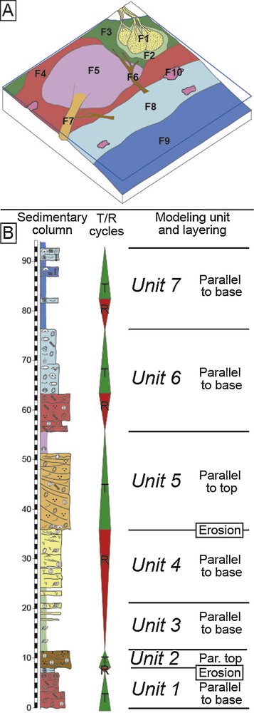
(Color online.) A. Conceptual depositional model for the Ilerdian Alveolina Limestone Fm. in the Serraduy area, showing the spatial distribution of depositional environments (See Fig. 2 for code). B. The sedimentary architectures and the sequence stratigraphy framework of the series were used to define the modeling units and the layering type for the subsequent modeling phase.
Based on (1) the vertical depositional environment stacking pattern, (2) the sedimentary architectures, (3) the recognition of major discontinuity surfaces, the studied succession was divided into several small-scale transgressive/regressive cycles (sensu Strasser and Hillgärtner, 1998), bounded by sedimentary discontinuities: sharp changes of facies, omission surfaces, erosional truncations (see Leturcq, 1999 for a discussion of the origin and duration of cycles). This sequential framework enables the sedimentary succession to be divided into modelling units that may correspond to entire cycles (units 1, 6 and 7) or part of them (units 2 and 5). In order to respect the sedimentary architectures, units 3 and 4 correspond to lithologic units rather than chronostratigraphic ones (Fig. 3). It enables to propose a unit layering that best fits the real geometries.
4 Diagenesis characterization
4.1 Diagenetic phase identification
The various diagenetic phases, including different types of cement, dissolution events, compaction and pressure-solution were identified, using staining of thin sections (Dickson, 1966), conventional and cathodoluminescence petrography. A general paragenesis describing the relative timing of these diagenetic phases is proposed in Fig. 4, mainly based on crosscutting relationships observed during petrographic analyses. The first diagenetic event occurring in the limestone facies is the micritization of bioclasts. It is attributed to micro-borer organisms living at or near the sediment-water interface (Purser, 1980), and is considered as almost syn-sedimentary. A selective dissolution of aragonite and high-magnesium calcite bioclasts (mainly gastropods and corals) is observed, resulting in a moldic porosity. The latter is completely occluded by a micritic infill, pointing at an early dissolution, and/or different cement phases (dogtooth isopachous fringes of Calcite 1, and a blocky to equant mosaic formed by Calcite 4). Recrystallization of micrite to microspar occurred in most of the samples. The microspar exhibits a crystal size from 5 to 20 μm, and shows a mottled aspect, dull orange luminescence. Numerous calcite cements were observed in the Alveolina Limestone Fm. (Figs. 4–6). The first one (Calcite 1) occurs mainly in grainstones (F6–F7) and wackestone facies (F4). It consists of a thin (5–20 μm thick) circumgranular fringe around grains (Fig. 6), or of a first generation of void-filling calcite (lining the pore). It is a non-ferroan calcite, with bladed to dogtooth crystals. There is no luminescence or a very dull luminescence. Calcite 2 is non-ferroan calcite cement, observed as (50 to 300 μm thick) syntaxial overgrowths around echinoid fragments, and occurring preferentially in bioclastic carbonate facies. It is composed of inclusion-rich crystals, showing frequent cleavage twins. It generally engulfs the cement 1. Under cathodoluminescence, the overgrowths are dull to non-luminescent. In some cases, a second generation of overgrowths, slightly luminescent with concentric zoning (orange), is observed around the first dull overgrowths. The third calcite (Calcite 3) is observed in the siliciclastic-dominated part of the sedimentary succession. It is pore-filling cement, with a possible equant mosaic texture. This calcite exhibits a mauve-purple color under potassium ferricyanide staining and shows dark orange to red luminescence (ferroan calcite). This cement is scarcely represented and followed by Calcite 4. The latter is a non-ferroan calcite, with a blocky to equant mosaic fabric (crystal size ranging from 75 to 200 μm), with a concentric zoning under cathodoluminescence, organized in fine concentric alternations (dull to light orange luminescence, Fig. 6) in the center, fading to a dull periphery. The zoning is not always well marked, and crystals sometimes appear unzoned. This cement was observed in the inter- and intraparticle porosity, in the moldic porosity, as infills of compaction microfractures. It also occludes the remaining space within the deformed and fractured Alveolina chambers or biomolds (thus postdating the mechanical compaction processes). Calcite 4 is also affected by bed-parallel stylolitization, predating the chemical compaction processes.
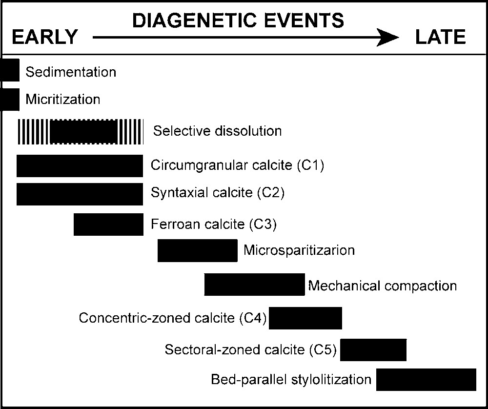
General paragenesis of the Alveolina Limestone Formation.
Modified from Hamon et al., 2012.
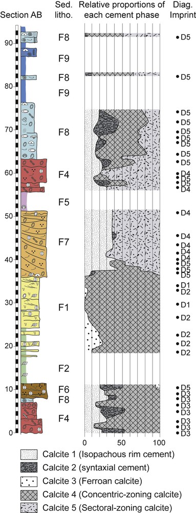
(Color online.) An example of vertical distribution of the different cement phases, quantitatively estimated by point counting on thin sections (section AB). Values are normalized to the total counted points of interstitial material (grains not counted). On the right, corresponding distribution of the different diagenetic imprints used for the modeling phase.
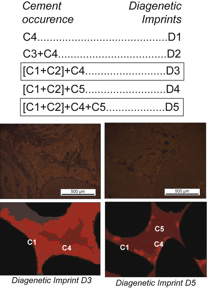
(Color online.) Definition of the diagenetic imprints used for the geostatistical simulations, grouping a succession of cement phases. Two examples (D3 and D5) are presented using cathodoluminescence photomicrographs to illustrate the sequence of successive cement phases.
Finally, a last non-ferroan calcitic cement (Calcite 5) is observed in the remaining intraparticle porosity and biomolds. It is made up of a druzy to blocky fabric with crystals ranging from 100 to 300 μm in size. This cement shows a sector zoning under cathodoluminescence (Fig. 6). It clearly postdates Calcite 4. Relationships between the stylolithisation and Calcite 5 are unclear as this cement can be locally affected by compaction stylolithes (syn-stylolithisation timing).
4.2 Spatial and stratigraphic distribution of cements
In this paper, the joint modeling of sedimentary and diagenesis trends aims at simulating both the distribution of sedimentary lithotypes and the cement phases, as they are the main phases that impact the reservoir properties. Indeed, the moldic porosity created by early selective dissolution stayed volumetrically low and was not considered.
For modeling purposes, the diagenetic phases described above needed to be quantified. This quantification of each cement phase was performed by point counting on thin sections, using JmicroVision Image analysis system (Roduit, 2008). The point counting was performed using a random selection of points, and stopped based on a stochastic criterion (when the percentages are getting stable, the counting can be stopped). An example of such quantification is presented for the sedimentary section AB in Fig. 5.
Calcite 1 is observed in each carbonate facies, in various proportions. It is mainly developed in grainstone facies (F6 and F7), around grains, and represents 20 to 40% of the total interstitial material (matrix and cement). Neither vertical gradient of cementation (from top to base of the megadune), nor lateral trends (along prograding sets) were observed. Calcite 1 is volumetrically insignificant in muddy facies (0 to 5%).
Calcite 2 (syntaxial overgrowth) is relatively scarce compared to the other cement phases (5 to 10% with one exception in section AB). The depositional facies exerts a strong control on the distribution of C2. Indeed, it is mainly observed in facies enriched in echinoid debris, in the topmost part of the series (F8 and F9).
Calcite 3 is only observed in the siliciclastic-dominated part of the series (F1), ranging from 0 to 20% of the total interstitial material. Moreover the quantity tends to decrease vertically (from base to top of the siliciclastic interval), which may reflect the progressive increasing distance from the source of fluids, i.e. clays. Calcite 4 is generally observed in the whole series, in various proportions (20 to 70% of the total interstitial material). However, a few exceptions are observed, specifically in F7, at the base of the Unit 5 (megadune, in sections AB, C, F, H, I). In this geobody, Calcite 4 is only present in the first two meters (from the base), progressively disappearing. A concomitant increase of Calcite 5 is observed.
Finally, Calcite 5 is only present in the upper part of the series, above the siliciclastic interval (units 3 and 4). Proportions are variable (5 to 70%) with a mean value around 15–20%. Its maximum development is associated with originally highly porous facies, with interparticular porosity (F7) or coral-dominated facies (F10).
4.3 Inputs for modeling
For modeling purposes, five “diagenetic imprints” were created. A diagenetic imprint is defined as a typical sequence of cements that affected one sedimentary lithotype (Fig. 6). For example, the diagenetic imprint D3 corresponds to the sequence of three successive cement phases: Calcite 1, Calcite 2 and Calcite 4 (Fig. 6). The proportions of diagenetic imprints, for each sedimentary lithotype, were estimated based on the quantification of each cement phase by petrographic analysis. For instance, F6 only shows diagenetic imprints D3 (with a proportion of 95%) and D5 (with a proportion of 5%). These association laws were defined for each sedimentary lithotype (Fig. 7).
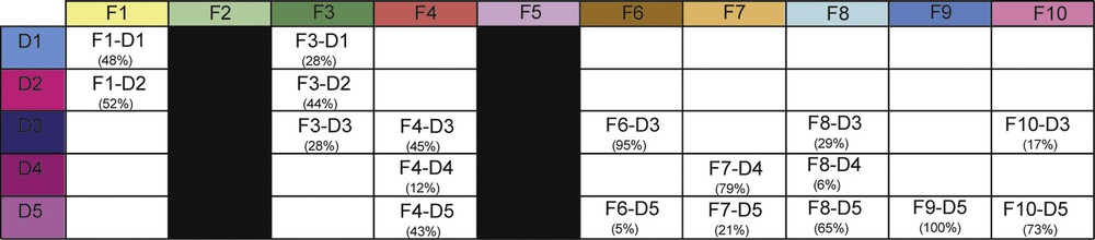
Quantified association laws defining the relationships between sedimentary lithotypes and diagenetic imprints.
5 Three-dimensional modeling
5.1 Modeling workflow
The previous dataset was used for stochastic modeling with CobraFlow, an in-house “IFP Énergies nouvelles” software. This software is designed to respect sequence stratigraphic constraints and to honor both the well data itself and its spatial variability. The model is 3 km long and 3 km wide, with a mean cell size of 10 m by 10 m horizontally and 1 m vertically. In the present study, the simulation workflow is based on the bi-plurigaussian (Bi-PGS) algorithm (Doligez et al., 2011, Pontiggia et al., 2010). The Bi-PGS model is a new model that enables two properties to be co-simulated with a large flexibility in the choice of the parameters characterizing each type of variable, and enables the heterotopic variables (i.e. corresponding to different datasets) to be taken into account. Each step of the workflow is performed sequentially: (1) cartography of the top and bottom of each unit, and creation of corresponding grids; (2) sedimentary lithotype simulation; (3) joint diagenetic imprint simulation.
The grid used for the simulation was divided vertically into seven units, the geometries of which are constrained by well markers. Each modeling unit is characterized by a specific layering, depending on its internal architecture (Fig. 3). The sedimentary lithotype simulation was performed using a first plurigaussian algorithm (non-stationary simulation), constrained with the ten sedimentary sections. Complex spatial relationships between depositional environments can be dealt (through “lithotype rules”) with using this software, and more geological information can be included (spatial trend and anisotropy, lateral discontinuity of lithotypes…). The diagenetic imprint simulation was carried out using a second plurigaussian algorithm. The computation of the parameters for this second simulation was conditioned by the association laws between sedimentary lithotypes and diagenetic imprints (Fig. 7). Using this second plurigaussian simulation means that a continuity in the diagenetic property from one cell to another can be obtained, even if the sedimentary lithotype changes between these cells (that would not be possible with a nested approach; Barbier et al., 2012; Doligez et al., 2011).
Thus, two independent simulations were produced, using two independent plurigaussian algorithms that are linked only through the computation of parameters and the conditioning data. Finally, the different realizations (sedimentary lithotypes and diagenetic imprints) are combined, to produce the joint simulation of both the sedimentary trends and the associated diagenetic imprints.
5.2 Choice and representativity of the geostatistical parameters
The simulation parameters for the plurigaussian lithotype simulation were defined with the outcrop analysis and the conceptual geological model. Main geostatistical parameters are: (1) the lithotype rules, (2) the vertical proportion curves (VPC) and the proportion matrix, and (3) the variogram models for the underlying Gaussian functions.
The plurigaussian algorithm requires the definition of lithotype rules that represent the possible vicinity between lithotypes. From a sedimentological point of view, it can be considered in a similar fashion to a facies substitution diagram (Homewood et al., 1992), which represents the possible lateral variations between the depositional environments. The number and the spatial distribution of sedimentary lithotypes being different from one unit to another, it was necessary to propose one lithotype rule for each modeling unit. These rules were built by integrating the stacking pattern and the spatial evolution of the sedimentary lithotypes defined previously.
For example, in modeling unit 3, four sedimentary lithotypes (depositional environments) coexist (Fig. 8A). Sandstone facies (F1) forming lobes and channels associated to their shaly fringes (F2) immediately downstream, and to a gastropod-rich sandy wackestone deposited in interdistributary restricted ponds (F3), are components of a small-scale deltaic complex under tidal influence. In the corresponding lithotype rule, these three lithotypes were organized together as they can pass laterally and vertically from one to another. F4 corresponds to Alveolina and Orbitolites dominated wackestone to packstone (shallow beach environment). It can be laterally equivalent to F2 and F3, away from clastic inputs, which were represented in the lithotype rule by a direct contact between these three lithotypes (Fig. 8A). As the spatial distribution of diagenetic imprints was difficult to assess from the petrographic study, only one Gaussian function with an ordered organization as default lithotype rule was used. The possible transitions between diagenetic imprints are constrained by the lithotype rules and association laws between sedimentary lithotypes and diagenetic imprints.
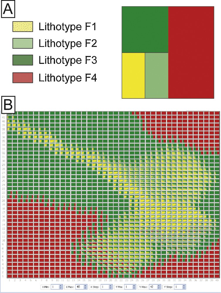
Two of the main parameters defined for the use of the plurigaussian algorithm. A. Lithotypes and lithotype rule defined for the third modeling unit. The latter parameter is based on the facies association relationship assessed from the depositional model (Fig. 3A). B. Corresponding proportions matrix, based on the vertical proportion curve computed from the ten sedimentary sections.
Moreover, vertical proportion curves (VPC) and proportion matrix (Doligez et al., 2011) were computed for each modeling unit. A VPC is a cumulative histogram of the proportions of the lithotypes present in the discretized wells. In other words, it represents the vertical succession and distribution of facies associations in one modeling unit. The VPC is computed from well data, at each stratigraphic level. When only one VPC is used as a parameter for the geological geostatistical simulations, the facies proportions are considered to be constant in average for each horizontal level (horizontal stationarity). The proportion matrix corresponds to the cases when proportions also vary laterally (3D non-stationarity in our case study). It is drawn as a 2D grid, each cell being itself a local vertical proportion curve (Doligez et al., 2011; Pontiggia et al., 2010; Ravenne et al., 2000), and reproduces the spatial variability of facies trends. For each modeling unit, a proportion matrix was computed from 10 vertical proportion curves (10 sedimentary sections), by level-by-level interpolation with a kriging method or ad hoc estimations, and a zoning based on the depositional model resulting from the sedimentological characterization (Fig. 8B). In order to co-simulate the diagenetic classes using also a plurigaussian approach and consistently with the lithotype distribution, a 3D matrix of vertical proportions related to the diagenesis has been computed. It was calculated from the sedimentary lithotype matrix (as constraint), using the global proportions (calculated from the data) of the diagenetic classes within each sedimentary facies. This allowed redistributing the diagenetic property according to the sedimentary lithotype proportions. For unit 2, a deterministic approach was used, as only one lithotype is involved.
Finally, in the plurigaussian algorithm (Le Loc’h and Galli, 1996), the facies simulation was performed using two stationary Gaussian random fields, which are truncated by using local thresholds computed from the lithotype rule, updated with the local proportions. Each Gaussian field imposes its spatial correlation structure to one or more of the facies, according to the defined threshold rule. In this study, we used Gaussian functions to define the variogram models of the two random fields, in order to generate smooth distributions of the facies. The ranges for the underlying Gaussian function are in relation with the distances of maximum correlation and spatial continuity of the sedimentary lithotypes. Thus, ranges vary from 100 m (patchy bioconstructions; F10) to 5 km (F4) in the horizontal directions and a few meters along the vertical axis, to be consistent with the continuity of the observed geological geometries.
6 Results and discussion
6.1 Simulation results
The joint simulation of both the facies associations and the diagenesis illustrates in three dimensions the extension and distribution of the different facies and heterogeneities that occur in each modeling unit. In our workflow, only the distribution of cement phases was modeled. Fig. 9 presents examples of sedimentary lithotype simulations throughout the whole interval of the Alveolina Limestone Fm. (modeling units 1 to 6). Fig. 10 shows an example of joint simulations of sedimentary lithotypes and diagenetic imprints for modeling unit 3.
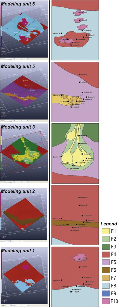
Sedimentary lithotype simulation results for different modeling units. These realizations are presented together with paleogeographic maps created independently during the sedimentological characterization phase and used as validation constraints.
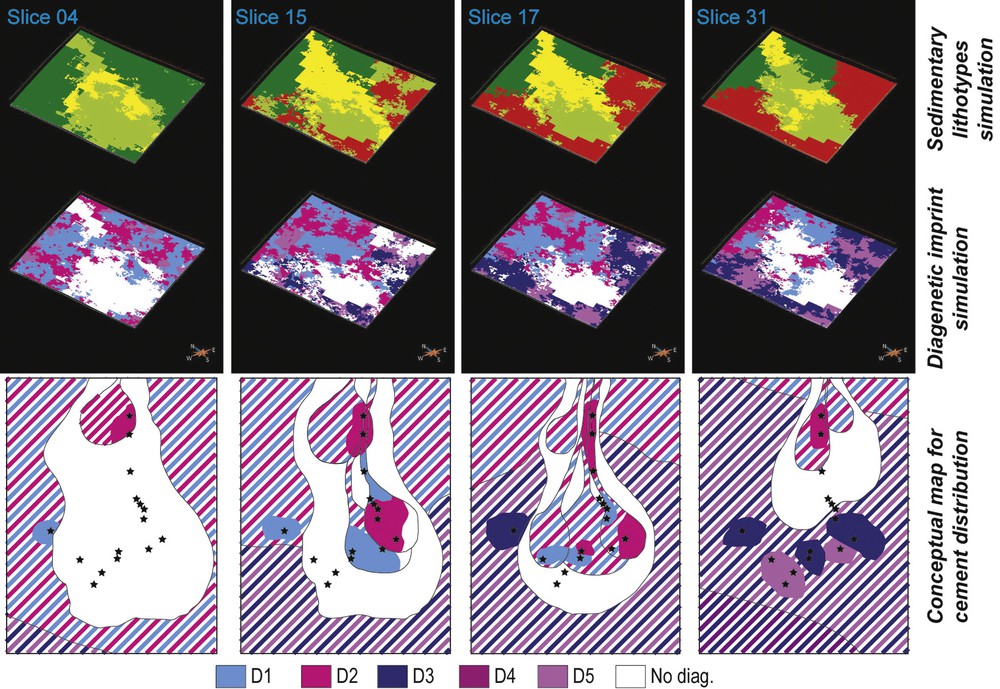
An example of joint simulation (sedimentary lithotypes and diagenetic imprints) for modeling unit 3. The figure shows a realization in facies and diagenesis for different levels of the unit. These realizations are presented together with “diagenetic maps” created independently during the diagenesis characterization phase and used as validation constraints. Hatched colors correspond to unsure, extrapolated areas from the constraining points (sections).
6.2 Validation of the simulations
The simulation results were validated by comparison with the conceptual geological model based on the field and petrographic observations described above.
The base of the series (modeling unit 1) is marked by a homogeneity of facies: shallow inner-ramp and mid-ramp deposits (F4 and F8) that cover the major part of the study area, with a local coral-dominated patch reef (F10). A tidal channel cuts through the previous inner platform deposits (F6; modeling unit 2). This facies distribution is well reproduced in the stochastic facies simulation (Fig. 9), that exhibits an homogeneous ramp sedimentation (F4–F8) with localized geobodies such as patch reefs (F10) and channels (F6).
The siliciclastic interval (modeling units 3 and 4) developed on these deposits, and is composed of at least seven sandy lobes (F1), supplied from the north by multiple distributary channels. Again the lithofacies simulations are consistent with this conceptual geological scheme. Indeed, the simulations correctly reproduce the channel/lobes complex that develops in a shallow, restricted environment (lithotypes F3–F4). Diagenesis simulations were performed in modeling unit 3 (Fig. 10). F3 is affected by diagenetic imprints D1, D2 and D3, whereas F4 is affected by D3, D4 and D5, and F1 is only affected by D1 and D2. F2 is a shaly facies, so no calcite cementation was observed, and no diagenetic imprint was simulated. These four lithotypes thus exhibit a high variability in terms of diagenetic imprints that increases the heterogeneity within this part of the series. The continuity of diagenetic imprints from one cell to the next one can be observed, even if the sedimentary lithotype is different between these cells. Compared to the cement distribution assessed from petrographic quantitative estimation, diagenetic imprints simulation seems to also correctly honor the geological model (Fig. 10).
The deltaic complex is overlain by lagoonal deposits (F5) that are themselves eroded at their top by a deeply scoured channel, filled by the large bioclastic prograding megadune (F7, modeling unit 5). It is drowned and covered by a homogeneous sedimentation of inner lagoonal deposits (F4), itself overlain by patchy bioconstructions (F10), interfingered with inner- (F4) to mid-ramp deposits (F8) (modeling units 6 and 7). In this unit, some slight discrepancies between the simulation and the paleogeographic map shown in Fig. 9 exist, which is due to the fact that the simulation slice is located in the topmost part of the unit, whereas the paleogeographic map summarizes information over the whole unit.
7 Conclusion
This study first demonstrates an innovative ability to account for the heterogeneity in the sedimentary facies distribution and the subsequent imprint of diagenetic facies during reservoir modeling. This study also shows the necessity to integrate the sedimentary and the petrographic analysis in the modeling workflow. A thorough description and quantification of both facies and diagenetic phases are necessary inputs for a valid geostatistical modeling of the reservoir's properties.
From a modeling point of view, the plurigaussian simulation used to populate the sedimentary lithotypes (equivalent to depositional environments) reflects the complex sedimentary architecture of the geological model and accounts for the spatial variability (non-stationarity) of each facies association. The joint simulation (Bi-PGS) allows us to constrain the spatial distribution of a specific diagenetic imprint, which is indirectly constrained in terms of timing of emplacement by the paragenetic sequence. It also allows us to account for a heterotopic set of data (data that are not systematically known at the same locations) for the conditioning step, as the simulations are independent.
The key parameters for the joint simulation, which leads to a consistent distribution of the main characteristics impacting the petrophysical properties in the studied reservoirs, are the following: (1) the quantification of the diagenesis variable, which needs to be improved through image analysis or multivariate statistics, (2) the definition of relationships between the sedimentary facies association and the diagenetic imprints.