

1 Introduction
In recent years, there has been an increasing global concern in protecting the biodiversity and water quality of marine and coastal waters. Such a concern is present for example in two key European parliament directives: the Water Framework Directive (WFD, Directive 2000/60/EC of 23 October 2000) and the Marine Strategy Framework Directive (MFSD, Directive 2008/56/EC of 17 June 2008). These have led to a greater number of marine protected areas, including seas, oceans, and lakes, all with the aim of protecting natural or cultural resources.
In the framework of such European directives, monitoring systems in coastal waters is essential in collecting information on physical, biogeochemical, and biological parameters. Many monitoring programs have been installed with weekly or monthly on-site sampling. Due in part to physical forcing, such as waves and turbulence, the marine environment is highly variable on smaller time scales. Consequently, several autonomous and automatic monitoring programs have been installed in recent years (Chang and Dickey, 2001; Chavez et al., 1997; Dickey, 1991; Dickey et al., 1993; Dur et al., 2007; Nam et al., 2005). These operate typically at 10 to 30 min time resolution at fixed position, corresponding to Eulerian sampling. There is a factor of about 1000 between sampling at 20-min resolution and sampling every two weeks. In the following, 20-min sampling resolution is referred to as “high frequency”. There are sensors able to measure physical or biogeochemical quantities at even higher frequencies (Seuront et al., 1999), but such systems have not been operating autonomously for several years.
Here we focus on the temporal variability of temperature using two data sets recorded at fixed locations along the French coastal area of the English Channel. The first one is a mooring, located in the western English Channel in the bay of Morlaix. The second is an automatic system called MAREL Carnot, located in the eastern English Channel at the exit of the harbor of Boulogne-sur-Mer. In both cases, the data from these automatic systems were recorded long-term (such denomination is usually used for record periods larger than about five years) using an automatic system at high frequency, with more than one measurement per hour.
High-frequency measurements at a fixed location correspond to an Eulerian sampling of a highly variable time-scale system. Sometimes such measurements are considered limited due to the fact that they provide a local view in time, where spatial information is lacking. Here, in order to have a view on the temporal and spatial link between two high-frequency measurement time series (recorded at two locations separated by several hundred kilometers), we shall study the correlation between the two series. The study of the multiscale correlations between these time series will provide us with the first hint at a spatialization of a time series at fixed locations. In this context, we will consider seven years of data, between 2005 and 2011, for two different temperature records. The following section presents the characteristics of these automatic systems, their datasets, and their climatology. We then proceed with showing some spectral and co-spectral analyses. The last section considers time dependent intrinsic correlation analysis of both time series–a new correlation method based on the empirical mode decompostion.
2 Data presentation and climatology
2.1 Estacade at Roscoff
The first of the two stations is considered here, where measurements of temperature were taken at the coastal site of Estacade (48°43.56 N, 3°58.58 W) located in the bay of Morlaix in the western English Channel (Fig. 1), from 2005 to 2011. In this area, characterized by strong tidal currents and tidal amplitude over 6 m, the water column remains completely mixed throughout the year. Temperature was measured with a sampling frequency of 10 min using a Seabird SBE39 recorder installed on a mooring at the sea bottom (mean water depth: 5.8 m). The percentage of available data for this period is close to 97%, which corresponds to 329,294 data points acquired (Fig. 2). The analytical precision of temperature measurements from the Seabird SBE39 sensor is 0.01 °C; the raw data at the output of this system are presented in Fig. 2 with a green pattern.
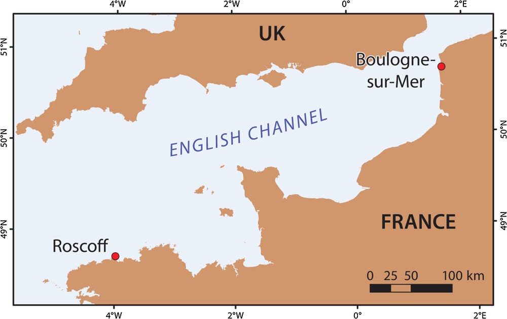
A map showing the measurement location in Boulogne-sur-Mer's coastal waters (France) at position 50°44.42 N, 1°34.06 W, in the eastern English Channel, and Roscoff (France) at the position 48°43.56 N, 3°58.58 W, in the western English Channel.
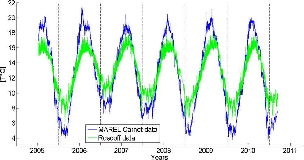
Temperature MAREL Carnot (Boulogne-sur-Mer) and Roscoff data series between 2005 and 2011. Vertical lines separate each year.
2.2 MAREL Carnot at Boulogne-sur-Mer
The second temperature datasets were recorded by an automatic system called MAREL Carnot, which is situated in the eastern English Channel in the coastal waters of Boulogne-sur-Mer (France) at position 50°44.42 N, 1°34.06 W (Fig. 1), with a periodicity of 20 min (see Zongo et al. (2011) for a presentation of this data set). Water depth at this position varies between 5 and 11 m; the measurements are taken using a floating system inserted in a tube, 1.5 m below the surface. Due to maintenance and failure of the automatic devices, there are several missing data. We consider here data from 2005 to 2011. The percentage of available data for this period is close to 88%, which corresponds to 138,574 data points acquired (Fig. 2). The MAREL Carnot station is included in the MAREL network (Automatic monitoring network for littoral environment, IFREMER, France), which is based on the deployment of moored buoys equipped with physicochemical measuring devices, working in continuous and autonomous conditions (Berthome, 1994; Blain et al., 2004; Dur et al., 2007; Schmitt et al., 2008; Woerther, 1998; Zongo and Schmitt, 2011).
2.3 Climatology
We consider here the climatology, i.e. the average inter-annual variations, estimated by averaging the data for each calendar day. This is shown in Fig. 3 for both temperature datasets, where the dotted lines represent upper and lower curves built using the standard deviation estimated over six different values (for a given calendar day) corresponding to the seven years of the study. The climatology of Roscoff shows a climate more maritime than in Boulogne-sur-Mer, which is more continental with warmer summers and colder winters. There is a minimum of around 9 °C and a maximum of around 16 °C, corresponding to an annual mean delta of 7 °C for Roscoff, while for Boulogne-sur-Mer it is close to 12 °C, with a maximum of around 18 °C and a minimum of around 6 °C. The two curves are quite smooth, showing a rather limited variability around this seasonal evolution. The standard deviation of the climatology, as presented in Fig. 3, is more important in the Boulogne-sur-Mer area. Therefore, the inter-annual temperature variations are less marked in the Roscoff area.
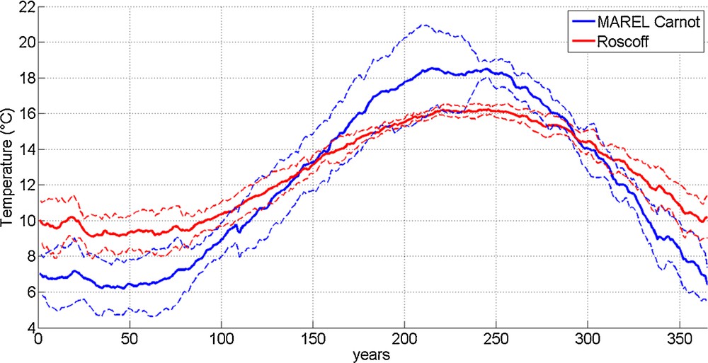
The climatology of both MAREL Carnot and Roscoff temperature data: inter-annual daily averages computed using the data from 2005 to 2011. The dotted lines represent the upper and lower limits estimated using their standard deviations; the latter being estimated over seven different values, estimated yearly from 2005 to 2011. Roscoff waters are more influenced by a maritime climate: winters are warmer and summers cooler.
3 Spectral analyses and co-spectra
We perform here spectral and co-spectral analyses. Fourier power spectra have been used in many previous studies in aquatic sciences over several decades to characterize scaling regimes (Legendre and Legendre, 2012; Platt and Denman, 1975; Seuront et al., 1996a,b; Seuront et al., 1999; Seuront et al., 2002; Winder and Cloern, 2010). To perform co-spectral analysis, a same time step is needed. Hence, for this analysis, a linear interpolation has been performed to degrade the time step to 20 min for the Roscoff dataset. Two spectra are shown in Fig. 4, in log–log plot. The spectra are clearly scaling, with slopes close to–5/3–as expected for passive scalar turbulence (Corrsin, 1951; Obukhov, 1949; Tennekes and Lumley, 1972). There are two peaks close to 12 h and 1 day, which are probably related to the impact of daily and tidal cycles. There are several slight peaks at high frequencies, and a larger peak around 90 days that could be related to the seasonal cycle.
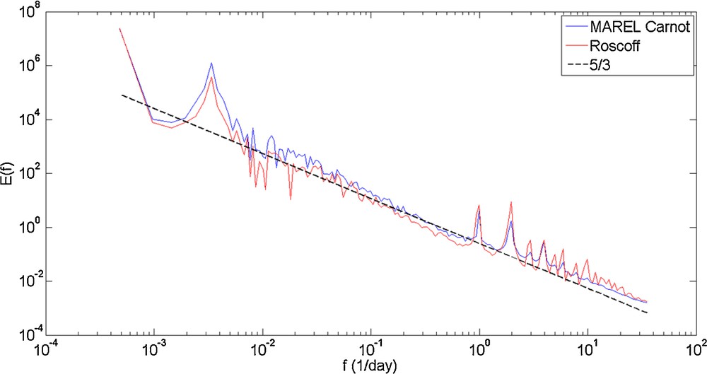
Fourier power spectra of Boulogne-sur-Mer (MAREL Carnot) and Roscoff temperature time series, and a 5/3 slope straight line for comparison, corresponding to passive scalar turbulence. Some peaks are visible, corresponding mainly to seasonal, daily, and tidal cycles.
3.1 Co-spectral analyses
In order to compare the two dynamics at different scales, we have estimated the co-spectrum, defined as (Bendat and Piersol, 2000):
| (1) |
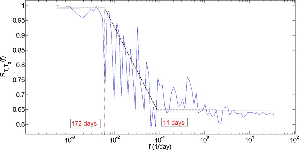
Co-spectra in semi-log (x axis) plot, of the temperature series in Roscoff and Boulogne-sur-Mer. There is a good correlation for scales larger than 172 days, a transition between 172 and 11 days, and a relative decorrelation for scales smaller than 11 days.
4 Time-dependent intrinsic correlation analysis (TDIC)
4.1 TDIC and EMD
We perform here a time–frequency analysis using Empirical Mode Decomposition (EMD), which was first introduced at the end of the 1990s in the field of physical oceanography (Huang et al., 1998, 1999). It has since been very successful with applications in many fields of science, and has received several thousand citations. The aim of this method is to decompose a time series in a sum of time series called “modes”, each having a characteristic frequency. At the end of the decomposition, the method expresses the analyzed signal X(t) as a sum of mode time series Ci(t) and a residual r(t):
| (2) |
| (3) |
| (4) |
Here to perform the TDIC method (Fig. 6), we used a Matlab code written by Yongxiang Huang (Huang and Schmitt, 2014); this code is itself based on the code written by Chen and Huang (Chen et al., 2010). The TDIC method has the advantage of giving a correlation for each characteristic scale, but for our time series with a time step of 20 min, it was not possible to enter directly the raw data, because of memory limitation to perform this computation. In this context, we have degraded our time series to perform the experiment reported in Fig. 6, where the new time step used is 1 day. This is not affecting information on time scales larger than one day, which are the concern here.
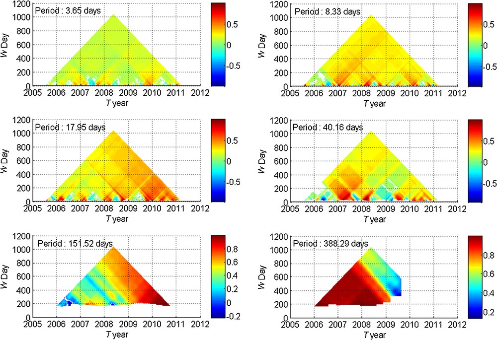
Cross-correlation plot between Roscoff and Boulogne-sur-Mer temperature series, using the TDIC method, based on empirical mode decomposition. The correlation is done here for modes having similar scales. The cross-correlation is time dependent (horizontal axis), and estimated over interval of increasing widths (vertical axis). Color scales emphasize strong events of correlation or anti-correlation.
4.2 Application of the TDIC method
Fig. 6 represents six TDIC graphs, with a characteristic time between 3.65 and 388.00 days. A pattern is visible on the first four TDIC graphs (until 40 days). For each year, on the baseline there is a blue patch in summer and a red patch in winter, which means that there is a correlation in winter and an anti-correlation in summer. Considering larger time lags, at the scale of 3 days (first graph) there seems to be no correlation. On the contrary, for scales of 8, 18, and 40 days (graphs 2, 3, and 4), the color scale images show global correlations between the two series. For years 2006–2008, the correlation is stronger at the scale of 40 days, whereas for scales 2009–2011 the correlation is stronger at the scale of 18 days. On the last graph with a scale of 388 days, there is a large red correlation patch on the left side and a blue no-correlation patch on the right side. This pattern could be because the amplitudes of the temperature signal are very close for years 2007 and 2008.
5 Discussion and conclusion
We have performed a comparison between two automated fixed-point systems located in the English Channel. Firstly, we have considered the climatology for both areas, and we have seen that Boulogne-sur-Mer was situated in a more temperate climate zone than Roscoff. Secondly, we have observed that both temperature spectral slopes were close to 5/3, which is the spectral slope of a passive scalar in fully developed turbulence. Finally, both correlation methods have converged toward a transition scale of 11 days for both series: scales smaller than 11 days are not correlated and larger scales possess some correlation.
The Roscoff system is installed on a bottom mooring, contrary to MAREL Carnot, which records data from the surface. Both sites are in coastal areas with strong tidal currents and consequently the water mass is thoroughly mixed. The spectral analysis in section 3 reveals that mean forcings, which seem to have an influence on temperature, are cycles linked to day/night, tidal, seasons, and high tides. These forcings are mainly controlled by astronomical mechanisms. Overall, the surface currents in the English Channel go east toward the strait, from the Atlantic to the North Sea. The surface temperatures from Roscoff could influence the surface temperature in Boulogne-sur-Mer, with a characteristic time of 11 days corresponding to an average transport time. From the results of co-spectral analysis, a link between both series was found for scales larger than 11 days, which is also the time scale found by considering a mean velocity of 0.5 m/s and a distance of 460 km. The TDIC analysis provided results consistent with this time scale. This new method is also useful to locally express correlation events. Here, we found that for scales from 8 to 40 days, there is a correlation in winters and an anti-correlation is summers.
Fixed-point systems provide temporal information. We can draw a parallel with the hypothesis proposed by Taylor in turbulence (Taylor, 1935), which allows the transformation of temporal information in the turbulence field on spatial information, when we know the mean velocity. In this context, we could compare the events recorded by automatic systems to the outputs of a numerical model. This could give us information to refine the model output. With an average current speed of 0.5 m/s in our study area and a sampling frequency of 20 min, we have a distance below 1 km: this scale is consistent with the spatial resolution of currently used models (Beaman et al., 2011; Lim et al., 2013; Wolanski and Kingsford, 2014). Another perspective is to consider a possible link with the NAO (North Atlantic Oscillation) variability, as performed in a recent study, where the authors considered the link between sea surface temperature and the NAO (Tréguer et al., 2014).
Acknowledgements
The region “Nord–Pas-de-Calais” (France) and the “Agence de l’eau Artois Picardie” are thanked for the financial support granted to Jonathan Derot's PhD thesis. IFREMER is acknowledged for access to MAREL data and Thierry Cariou for access to Estacade data; we thank Alain Lefebvre and Michel Repecaud from IFREMER for discussions. Yongxiang Huang is thanked for discussions on the TDIC method. We thank Denis Marin (LOG) for realizing Fig. 1. The TDIC code is free to access on the following website: http://www.fg-schmitt.fr/EMD_and_multifractals.html. www.englisheditor.webs.com is also thanked for its English proofing.