Seismic random noise elimination according to the adaptive fractal conservation law

Fanlei Meng; Yue Li; Qian Zeng

doi:10.1016/j.crte.2015.12.002

Internal Geophysics

Seismic random noise elimination according to the adaptive fractal conservation law

Présenté par : Handled by Michel Campillo

Fanlei Meng ¹ ; Yue Li ² ; Qian Zeng ³

¹ Changchun University, School of Electronic and Information Engineering, Changchun 130022, China
² Jilin University, Department of Communication Engineering, Changchun 130012, China
³ Changchun Institute of Applied Chemistry Chinese Academy of Sciences, State Key Laboratory of Electroanalytical chemistry, Chuangchun 130022, China

Comptes Rendus. Géoscience, Volume 348 (2016) no. 5, pp. 350-359.

Résumé

The fractal conservation law (FCL) is based on the Cauchy problem of the partial differential equation (PDE), which is modified by an anti-diffusive term of lower order. The analysis indicates that it can eliminate the high frequencies and preserve or amplify the low/medium frequencies. The performance of FCL depends on the threshold selected for the PDE. This threshold corresponds to the cut-off frequency of FCL in the frequency domain. Generally, the threshold is fixed. Thus, the FCL cannot track the signal beyond the cut-off frequency, and it removes the higher-frequency components of the signal. To solve this problem, an adaptive FCL filtering method is presented. The main purpose of this method is to select the optimal FCL threshold in each sample index such that it can adaptively track the rapid changes in the signal. In the adaptive FCL, we select FCL estimations with different thresholds and construct a convex hull of these estimations of each sample index. Consequently, we introduce a quadratic functional with respect to FCL estimation to ensure that we select the optimal estimation from the convex hull of each sample index. This leads to a box-constrained convex problem, which can be solved by the Viterbi algorithm.

Métadonnées

Reçu le : 2015-11-30
Accepté le : 2015-12-10
Publié le : 2016-03-08

DOI : 10.1016/j.crte.2015.12.002

Mots clés : Adaptive filtering, Convex sets, Fractal conservation law (FCL), Partial differential equations (PDE) filters, Viterbi algorithm

Affiliations des auteurs :

Fanlei Meng ¹ ; Yue Li ² ; Qian Zeng ³

@article{CRGEOS_2016__348_5_350_0,
     author = {Fanlei Meng and Yue Li and Qian Zeng},
     title = {Seismic random noise elimination according to the adaptive fractal conservation law},
     journal = {Comptes Rendus. G\'eoscience},
     pages = {350--359},
     publisher = {Elsevier},
     volume = {348},
     number = {5},
     year = {2016},
     doi = {10.1016/j.crte.2015.12.002},
     language = {en},
}

TY  - JOUR
AU  - Fanlei Meng
AU  - Yue Li
AU  - Qian Zeng
TI  - Seismic random noise elimination according to the adaptive fractal conservation law
JO  - Comptes Rendus. Géoscience
PY  - 2016
SP  - 350
EP  - 359
VL  - 348
IS  - 5
PB  - Elsevier
DO  - 10.1016/j.crte.2015.12.002
LA  - en
ID  - CRGEOS_2016__348_5_350_0
ER  -

%0 Journal Article
%A Fanlei Meng
%A Yue Li
%A Qian Zeng
%T Seismic random noise elimination according to the adaptive fractal conservation law
%J Comptes Rendus. Géoscience
%D 2016
%P 350-359
%V 348
%N 5
%I Elsevier
%R 10.1016/j.crte.2015.12.002
%G en
%F CRGEOS_2016__348_5_350_0

Fanlei Meng; Yue Li; Qian Zeng. Seismic random noise elimination according to the adaptive fractal conservation law. Comptes Rendus. Géoscience, Volume 348 (2016) no. 5, pp. 350-359. doi : 10.1016/j.crte.2015.12.002. https://comptes-rendus.academie-sciences.fr/geoscience/articles/10.1016/j.crte.2015.12.002/

Version originale du texte intégral

1 Introduction

In land seismic exploration, the reflection events are used to characterize rock properties for surveying oil and gas resources. However, the contamination of seismic data with noise greatly degrades the geological information and hinders further processing. Usually, noise can be generated by various sources (e.g., wind and swell) and classified as two categories: coherent noise and incoherent noise. Unlike coherent noise, the incoherent noise is unpredictable in space and time that possesses randomness, and as the complexity of the geological conditions increases. In complex geological condition, for example in the mountainous areas in Northeast China, where storm weather covers more than six months of a year and among which five months suffer from severe winter storm. Then the random noise in the seismic record becomes more powerful and complicated (Wu et al., 2014). Therefore, the noise attenuation is an essential step for the seismic data analysis. In this paper, the removal of incoherent or random noise is our main focus.

Many methods in a variety of different fields have been developed to improve the signal-to-noise ratio (SNR) of seismic data by removing random noise, such as f–x deconvolution (Canales, 1984), frequency-spatial prediction (Wang, 1999, 2002), wavelet transform (Cao and Chen, 2005), polynomial approximation (Lu et al., 2006), and singular value decomposition (Lu, 2006). These techniques are often effective to mitigate random noise, but when the SNR is below a given threshold (for example, 0 dB), they no longer exhibit good performance. Some useful information, such as the relative maxima or minima of the signal, can be masked by these methods.

The fractal conservation law (FCL) filtering method (Azerad et al., 2012), which is simply the forward heat equation modified by a fractional anti-diffusive term of lower order, has been successfully applied for seismic data denoising (Meng et al., 2014, 2015) and was demonstrated to exhibit good performance compared to time-frequency peak filtering (TFPF) (Boashash and Mesbah, 2004; Roessgen and Boashash, 1994). By using an integral formula, which is based on Taylor-Poisson's formula and Fubini's theorem for an anti-diffusive term, and then taking the Fourier transform of the equation, the frequency response can be derived. The study showed that this response eliminates the high frequencies, amplifies the medium frequencies and preserves the low frequencies. The numerical computation based on the Fourier transform scheme runs fast, which is very conducive to practical application. However, there is a pair of contradictions in selecting the threshold frequency for filtering. If we choose a high threshold for filtering, it allows good preservation of the signal components but relatively poor random noise reduction, and because FCL can amplify the medium-frequency components, both the noise components and the signal with this frequency are also amplified. Conversely, if we choose a low threshold for filtering, effective random noise reduction is achieved, but the signal frequency components exceeding the threshold frequency are attenuated. Therefore, the conflict between signal preservation and noise attenuation cannot be resolved using a fixed threshold.

In this paper, we utilize a group of frequency responses (at least two responses) of FCL determined using different parameters to construct a convex hull (upper and lower bounds) of the filtering results. Then, we take the filtering convex set for each sample index and choose an optimal estimation with respect to time to minimize a given quadratic functional. Thus, adaptive FCL is equivalent to a convex optimization problem with box constraints (Boyd and Vandenberghe, 2004), which can be solved using the Viterbi algorithm (Todd and Wynn, 2000). The idea of this adaptive method was first introduced by Zeng et al. (2015). The recovery of seismic events using our algorithm is presented here. The experiments illustrate that the adaptive FCL is better than conventional approaches for random noise reduction and signal preservation.

The rest of this paper is organized as follows. Section 2 introduces the basic theories of the FCL method. In Section 3, we describe the proposed adaptive FCL method in detail. The performance of the novel approach is tested using both synthetic and field data and is compared with the performance of conventional FCL and other well-known denoising methods in Section 4. Finally, Section 5 concludes the paper.

2 Theory and computation of the FCL method

In this section, we provide a brief review of the theory of the FCL method and analyze its frequency response. The FCL method is based on the Cauchy problem of the linear partial differential equation (PDE), with two antagonistic terms: a common Laplace diffusion term $- \partial_{x x}^{2}$ and a nonlocal anti-diffusive term $I_{λ}$ of lower order (Azerad et al., 2012). The PDE is implemented on seismic data trace by trace and is given by:

\{\begin{cases} \partial_{t} y (t, x) - a \partial_{x x}^{2} y (t, x) + b I_{λ} [y (t, x)] (x) = 0, t \in (0, T), x \in R, \\ y (0, x) = s (x), x \in R \end{cases}

(1)

where y = y(t, x) is the filtered signal and s(x) is the initial signal, which is the noisy seismic signal. t is merely a parameter, whereas x represents the time of one seismic trace. T, a and b are positive constants, and

I_{λ}

is a fractional operator defined as follows for

λ \in (1, 2)

I_{λ} [y] (x) = α_{λ} \int_{R} \frac{y'' (x - ε)}{{|ε|}^{λ - 1}} d ε,

(2)

where

α_{λ}

is a suitable constant, and the double apostrophe denotes twice differentiation with respect to time. By using an integral formula for the anti-diffusive term, which is based on Taylor–Poisson's formula and Fubini's theorem, and then taking the Fourier transform of the PDE, the solution of (1) can be derived as (Azerad et al., 2012):

y (t, x) = k (t, x) * s (x),

(3)

where

*

represents convolution and

k (t, x) = F^{- 1} (K_{a, b}^{λ} (t, ω))

is the kernel of the operator

I_{λ} - \partial_{x x}^{2}

and

K_{a, b}^{λ} (t, w) \exp (- t (4 π^{2} a ω^{2} - b {|ω|}^{λ})) .

(4)

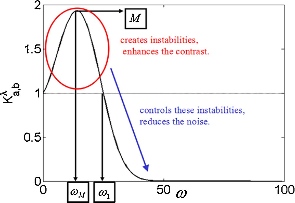
Equation (4) is the frequency response of the FCL method, and ω represents the frequency. Thus, the filtering process can be realized in the frequency domain for computational efficiency. Finally, by applying the inverse Fourier transform, we obtain the estimated value y(x) from the frequency domain into the time domain. To facilitate the calculation, t can be fixed at a value of 1. We draw $K_{a, b}^{λ}$ in Fig. 1 and note that the $- {|ω|}^{λ}$ is the symbol of the nonlocal anti-diffusion operator $I_{λ}$ , which creates instabilities and enhances the contrast. Conversely, the term 4π²ω² corresponds to the diffusion operator $- \partial_{x x}^{2}$ , which controls these instabilities and reduces the noise. Of course, the amount of denoising and enhancement are variable and are quantified by the parameters a and b, respectively. Hence, signal enhancement and denoising are not antagonistic.

Fig. 1
The behavior of $K_{a, b}^{λ}$ with 4π²a = 0.01, b = 0.05 and λ = 1.5.

As seen in Fig. 1, there are three important values regarding the choice of parameters a and b. One is the threshold frequency $ω_{1}$ , which satisfies $K_{a, b}^{λ} (ω_{1}) = 1$ and $K_{a, b}^{λ} (ω) < 1$ for $ω > ω_{1}$ . Two additional important values are $ω_{M}$ and M. We can obtain $ω_{M}$ by taking the derivative of $K_{a, b}^{λ}$ , and M is the maximum of $K_{a, b}^{λ}$ . Therefore, we deduce that $ω_{1}$ controls the frequency range to amplify; M can be interpreted as the amplification factor of the intermediate frequency. From (2), because $λ \in (1, 2)$ , setting parameter λ to be a fixed value is sufficient. We set λ as 1.5 for all experiments in this paper. According to the actual situation, we give a fixed value of $ω_{1}$ and M, which can, in turn, be used to determine the parameters a and b. For more details on choosing the parameters, we refer the reader to (Meng et al., 2015) and (Azerad et al., 2012), who provide an explicit discussion of this issue.

Fig. 2 shows the behavior of the frequency response $K_{a, b}^{λ}$ for fixed $ω_{1}$ and different values of M. It must be noted that as the value of M decreases, the decline in the relative high frequency will occur more slowly. Ignoring both the noise-reducing and contrast-enhancing abilities of this method and considering only its denoising ability, we can set the M to a smaller value (greater than but close to 1) and $ω_{1}$ to be relatively small. This is a compromise solution.

Fig. 2
Evolution of the frequency response $K_{a, b}^{λ}$ for different parameters.

3 Adaptive algorithm for FCL

Corresponding to the linear mapping $K_{a, b}^{λ}$ → y (boldface letter y is equivalent to y(x) in equation (3)), we let Y ={y} be a set of signals recovered by FCL filtering. Take u = sup{Y} and l = inf{Y} as the upper bound and the lower bound of Y at each sample index i, respectively. Then, the continuum and bounded convex set conv(Y_i) at each sample index can be constructed as follows:

c o n v (Y_{i}) = [l_{i}, u_{i}] = [\min {y_{i}, K_{a, b}^{λ}}, \max {y_{i}, K_{a, b}^{λ}}] .

(5)

where y_i

\in

[l_i, u_i] and our purpose is to identify the optimal y to minimize a strictly convex functional defined over an existing area Ω = {y, l ≤ y ≤ u}.

We applied the following quadratic functional as the convex optimization problem (Zeng et al., 2015):

J (y) = {∥A (y - s)∥}^{2} + {∥B (Dy)∥}^{2}, y \in Ω .

(6)

The || • || denotes the l₂(Ω) norm; A, B $\in$ Rⁿ ^× ⁿ are nonnegative diagonal parameter matrices, which enable (6) to track the magnitude attenuation of both signal and noise; and D $\in$ R ⁽ⁿ⁻¹⁾ ^× ⁿ is a difference matrix with the form:

D = [\begin{array}{c} - 1 & 1 & \dots & 0 \\ ⋱ & ⋱ \\ 0 & \dots & - 1 & 1 \end{array}]

The upper bound for the filtering error within Ω at the sample index i is (Zeng et al., 2015):

\max (u_{i} - y_{i}, y_{i} - l_{i}) \leq u_{i} - l_{i} = w_{i} + κ ψ_{i}, κ > 0,

(7)

where w_i is the maximum magnitude of the attenuation of the signal and

ψ_{i} = σ (∥K_{u_{i}}∥ - ∥K_{l_{i}}∥)

is the average magnitude of the attenuation of noise.

K_{u_{i}}

and

K_{l_{i}}

denote the filters

K_{a, b}^{λ}

at the boundaries of Ω, and the estimation of the standard deviation of the noise is given by (Zeng et al., 2015):

σ = Median (|s_{i} - s_{i - 1}, i = 2,3,..., n|) / 0.6745 .

(8)

According to the analysis above, A and B are assigned by

\begin{array}{l} {(A)}_{i, i} = ||u_{i} - l_{i}| - ψ_{i}| \\ {(B)}_{i, i} = κ ψ_{i} . \end{array}

(9)

Thus, with no a priori information regarding the noise-free signal, we know all the variables in objective function J(y), and it is possible to find the optimal solution y. The Viterbi algorithm, which shows good numerical stability, is suitable in this case.

We construct a trellis diagram with weights for adaptive FCL, which is illustrated in Fig. 3. The column S_i is called a stage, and each point in S_i is called a node. The values of the nodes at every sample index i are assigned by dividing the closed interval [l_i, u_i] into (N–1) equal sections:

S_{i} = \{y_{j, i} : y_{j, i} = l_{i} + j (u_{i} - l_{i}) / (N - 1), j = 0,1,2 \dots N - 1\} .

(10)

Fig. 3
Trellis diagram for adaptive FCL.

An edge is a connection between two nodes y_p,i and y_q,i+1 (p, q =0, 1, 2,…, N–1) in two stages S_i and S_i+1; the direction is from i to i + 1 (as indicated by arrows) and represents a transition to a new state at the next time instant. According to (6)–(9), the length of each edge is weighted by the metric:

{(A)}_{i, i}^{2} {(y_{p, i} - s_{i})}^{2} + {(B)}_{i, i}^{2} (y_{p, i} - y_{q, i - 1}) .

(11)

The cost of a path is the sum of the weights along the path from stage S₁ to S_n (n is the amount of the samples). We apply the Viterbi algorithm to identify the shortest path (survivor path) y to minimize the cost, which are computed according to the objective function in (6). That is to say, at each stage S_i, the estimation value (node) y_j, _i is optimal and adaptive. In fact, the choice of y_j, _i is equivalent to the choice of an optimal frequency response for each data point. The main strategy of the adaptive method is to select a low threshold frequency where the signal changes smoothly or the local SNR is relatively low; otherwise, a high threshold frequency will be selected. As a result, it not only effectively attenuates the random noise but also preserves the amplitude of the valid signal.

4 Application to seismic records

First, we present a synthetic seismic trace to better illustrate the adaptive performance of our method. As illustrated by Fig. 4a, the ideal signal contains three Ricker wavelets, whose dominant frequencies are 60, 40 and 20 Hz; and the sampling frequency is 1000 Hz. A white Gaussian noise (WGN) of 5 dB is added to this ideal signal. Fig. 4b shows the filtering results using the FCL method with different parameters. When the threshold frequency is set to 60 Hz (M = 1.05), we observe that the peak and the trough of each wavelet in the filtered signal are well preserved, but the denoising ability is relatively poor. Conversely, when the threshold frequency is set to 20 Hz (M = 1.05), we can see that the FCL method can effectively reduce the random noise but results in a serious attenuation of the signal amplitude.

Fig. 4
a: Noisy signal and ideal signal; b: filtering results by conventional FCL with different parameters; c: waveform comparison of ideal signal, FCL filtering signal and adaptive FCL filtering signal; d–f: partial enlarged images of each wavelet.

In Fig. 4c, we select a threshold frequency of 40 Hz as a compromise threshold for the whole data set (M = 1.05) using the conventional FCL method. For the proposed adaptive FCL method, we choose two filters with different threshold frequencies and M values. The two group parameters are {75 Hz, 1.2} and {15 Hz, 1.05}. Clearly, our method better attenuates the random noise and preserves the local extremum, especially for the high-frequency wavelet (60 Hz), which exhibits large amplitude attenuation after the FCL filtering. The detailed comparison of the filtering results in Fig. 4d–f highlights these points.

Second, we synthesize a seismic model that consists of two reflection events with linear and curving shapes. In Fig. 5a, there are 40 traces with 600 samples in each channel, and the sampling interval is 0.002 s. The seismic wavelets of the two events are modeled by Ricker wavelets with the dominant frequencies of 35 and 20 Hz, respectively. The SNR of the noise data in Fig. 5b obtained by adding random noise to the noise-free synthetic data is 0 dB. We process the noisy data using the wavelet-denoising method, F–X deconvolution, the FCL method and the adaptive FCL method trace by trace. The threshold frequency and the M value in the FCL method are set as 25 Hz and 1.1, respectively. For the adaptive FCL, we also choose two filters with the following two group parameters: {50 Hz, 1.05} and {7 Hz, 1.05}. The wavelet-denoising method uses the soft threshold approach with detailed coefficients obtained from the decomposition of the seismic traces at level 3 by the db4 wavelet (Lin et al., 2013, Tian et al., 2014). A comparison of the results obtained by using the wavelet method, F–X deconvolution method, FCL method and adaptive FCL method is shown in Fig. 5c–f. We can see that the wavelet-denoising method, the F–X deconvolution method and conventional FCL can suppress some of the random noise, but their denoising results are not satisfactory. Moreover, the shallow layer event is seriously attenuated. Conversely, a larger amount of noise is removed by the adaptive FCL method, and the two events are thus more clearly recovered.

Fig. 5
Example of a synthetic seismic model. a: Clean record; b: noisy record with a SNR of approximately 0 dB; c: record filtered using the wavelet-transform denoising method; d: record filtered using the F–X deconvolution method; e: record filtered using the FCL method; f: record filtered using the adaptive FCL method.

We extract time windows around the arrivals in the 41st trace derived from the above six records for a further comparison. From Fig. 6a and b, it can be observed that the amplitudes of the two wavelets are closer to the original signal and that the random noise is significantly lower when the adaptive FCL method is used compared to when the other three methods are used. Figs. 6c and d present a comparison of the 41st trace of the synthetic record in the frequency domain. We observe that the filtered signal after the wavelet-denoising method and the F–X deconvolution method are used exhibits a serious distortion in the low/medium-frequency components. To preserve the signal, regardless of the choice of $λ \in (0, 2)$ , the FCL filtering method will always amplify the medium-frequency components. Therefore, both the noise components and the valid signals in this frequency range will be preserved or even amplified. As presented in Fig. 6 (c, red line), because the threshold frequency is set as 25 Hz, the FCL method actually struggles to denoise the frequencies at 0–25 Hz. Once that threshold is exceeded, the filtered signal begins to decrease. This result is caused by a shortcoming of the conventional algorithm itself. This shortcoming is effectively resolved by using the adaptive method, which can track the rapid change in the waveform in both the time and frequency domains. We observe in Fig. 6c and d that the adaptive FCL method (blue line) provides an amplitude spectrum that is a good match to the noise-free spectrum for the signal components in the low/medium-frequency band.

Fig. 6
Waveform and spectrum comparison of the four methods in the 41st channel. a and b: Waveform comparison of the shallow and deep layer signals (35 and 20 Hz), respectively; c and d: spectrum comparison of the shallow and deep layer signals (35 and 20 Hz), respectively.

For the quantitative comparison of the denoising and signal-preserving abilities, we utilize the following formula to compute the SNR and mean square error (MSE) after adding different levels of WGN, as listed in Table 1. Correspondingly, Fig. 7a and b present the curves of SNR and MSE drawn based on the data shown in Table 1.

S N R (dB) = 10 \log_{10} (\frac{\sum_{i = 1}^{N} \sum_{j = 1}^{M} u_{0} {(i, j)}^{2}}{\sum_{i = 1}^{N} \sum_{j = 1}^{M} {(u_{0} (i, j) - u (i, j))}^{2}})

(12)

M S E = \frac{1}{M N} \sum_{i = 1}^{N} \sum_{j = 1}^{M} {(u_{0} (i, j) - u (i, j))}^{2} .

(13)

where u₀ is the noiseless original signal, u is the filtered signal, and N and M are the input matrix dimensions (Baddari et al., 2011).

Original record (dB)	Wavelet-denoising record	F–X deconvolution filtered record	FCL filtered record	Adaptive FCL filtered record
	SNR (dB)	MSE	SNR (dB)	MSE	SNR (dB)	MSE	SNR (dB)	MSE
10	13.3316	9.0969e-04	6.2854	0.0046	11.0850	0.0015	17.9123	3.1683e-04
5	9.3281	0.0023	5.8873	0.0051	9.3674	0.0023	13.1925	9.3929e-04
0	4.6998	0.0057	4.9872	0.0062	6.3824	0.0045	7.1127	0.0038
–5	1.8848	0.0127	3.4967	0.0088	2.1561	0.0119	3.6507	0.0085

Fig. 7
a: SNR values in the wavelet-transform denoising method, F–X deconvolution method and FCL method in comparison to the proposed method; b: MSE values in the wavelet-transform denoising method, F–X deconvolution method, and FCL method in comparison to the proposed method.

Through observation and comparison using Table 1 and Fig. 7, we know that the SNR is higher after filtering by adaptive FCL and that the MSE is smaller than those of the other three denoising methods. This is a consequence of the better estimation of the waveform by the adaptive method in both the time and frequency domains compared with the other three methods.

Third, we synthesize a more complex seismic model that consists of horizontal and slant linear events, hyperbolical events, broken events, and conflicting events, as shown in Fig. 8a. There are 80 traces with 2300 samples in each channel, and the sample frequency is 1000 Hz. The dominant frequencies of the reflection events are from 50 to 12 Hz. To more accurately simulate the real situation, in this example, we add real seismic pure noise, which was obtained from an actual seismic record in the Daqing area in Northeast China, to the synthetic model. We utilize the formula (12) to determine that the SNR of the noisy seismic data is approximately −4.56 dB, as shown in Fig. 8b. As seen, the continuity of the seismic reflection events is totally hidden in the real seismic noise. We process the data using the wavelet-denoising method, the F–X deconvolution method, and FCL and adaptive FCL methods, and the results are shown in Fig. 8c–f, respectively. The threshold frequency and the value of M in the FCL method are set as 30 Hz and 1.05, respectively. For the adaptive FCL, we also choose two filters with two group parameters: {55 Hz, 1.2} and {6 Hz, 1.05}. It should be noted that the events in Fig. 8 c, d and e exhibit a serious distortion, especially the shallower events. For the F-X deconvolution, some events can hardly be identified. Conversely, Fig. 8f shows that the adaptive FCL results in the cleanest background among the tested methods, allowing the events to be identified easily. The SNR of the wavelet denoising is approximately 2.72 dB, that of the F–X deconvolution filtering is approximately 3.94 dB, that of the conventional FCL filtering is approximately 3.18 dB, and that of the adaptive FCL filtering is approximately 4.11 dB.

Fig. 8
Example of a synthetic seismic model. a: Clean record; b: noisy record (SNR = –4.56 dB) contaminated with real seismic noise; c: record filtered by the wavelet-denoising method; d: record filtered by the F–X deconvolution method; e: record filtered by the FCL method; f: record filtered by the adaptive method.

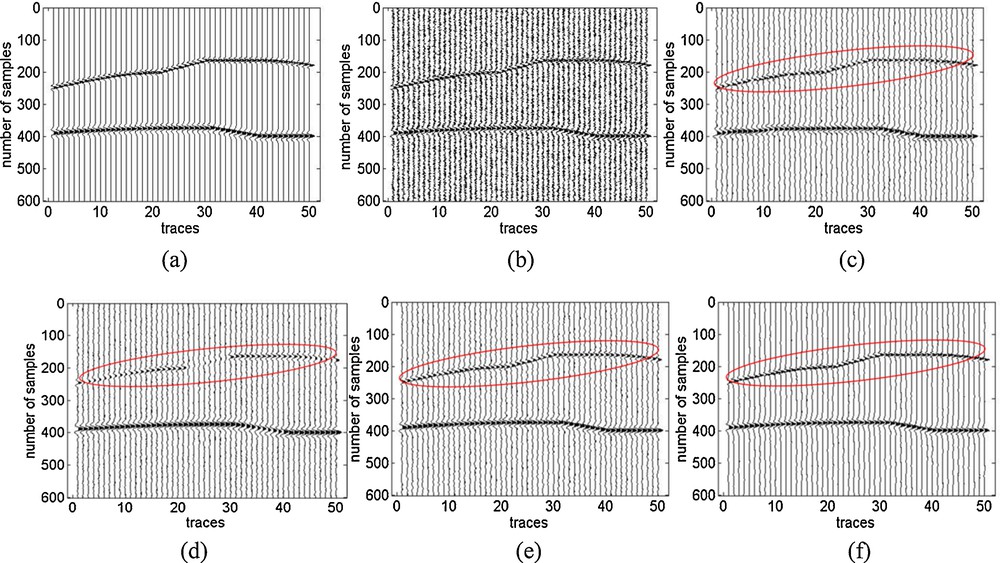
Finally, to verify the versatility of the proposed method, we test it on a common shot point seismic record, as shown in Fig. 9a. This record is a 4-ms sampling with 168 channels. The vertical axis represents the sampling time, and the horizontal axis represents the seismic trace. This record contains both hyperbolic events and approximately linear events, and the shapes of these events are different and irregular. The continuity of some of the seismic reflected events is obscured by the interference of random noise. Fig. 9b–e show the results of the F–X deconvolution method, the wavelet-denoising method, and the conventional and adaptive FCL methods, respectively. The threshold frequency and the M value for the FCL are set as 25 Hz and 1.1, respectively. For the adaptive FCL, we also choose two filters with two group parameters: {100 Hz, 1.2} and {5 Hz, 1.05}. It can be seen that the F–X deconvolution, wavelet-denoising and conventional FCL methods cannot reduce random noise as effectively as the adaptive FCL method. Moreover, Fig. 9b shows that the frequency of the valid signals varies (the reflection events become fatter) and that some details are lost. Compared with the conventional FCL, F-X deconvolution and wavelet-denoising methods, Fig. 9e shows better results, presenting better filtering performance regarding noise reduction and events preservation in the field seismic data. For a detailed comparison, we magnify the records between traces 27 and 148 and sampling time from 4404 to 7200 ms, as indicated by the rectangles shown in Fig. 9. The magnified areas are shown in Fig. 10. Again, as seen from Fig. 10b–e, our method was able to suppress the seismic random noise more effectively and recover the valid information more clearly and continuously than the other methods tested. We indicate these improved features with ovals.

Fig. 9
a: Real seismic record; b: record filtered using the F–X deconvolution method; c: record filtered using the wavelet-denoising method; d: record filtered using the FCL method; e: record filtered using the adaptive FCL method.

Fig. 10
Partial magnified images from Fig. 9: a: Unfiltered, magnified record; b: filtered, magnified record with the F–X deconvolution method; c: filtered, magnified record with the wavelet-denoising method; d: filtered, magnified record with the conventional FCL method; e: filtered, magnified record with the adaptive FCL method.

5 Conclusion

An adaptive FCL filtering method for the elimination of seismic random noise is proposed in this article as an improvement of the conventional FCL method. The threshold frequency has a significant effect on the filtering results of the FCL. The conflict between noise suppression and signal preservation cannot be resolved by a fixed threshold frequency. In the proposed method, the optimal estimation can be chosen from a convex set to minimize a convex functional. Therefore, this method further reduces the bias of the FCL filtering method for the estimation of seismic events. Experiments on both synthetic and field seismic data, including both qualitative and quantitative analyses, demonstrated that the new method is superior to the conventional FCL method and achieve both better random noise reduction and higher continuity and clarity of the reflection events.

Acknowledgments

We would like to thank the original authors of the FCL method, which is an important step forward in seismic signal processing. This work was supported by the National Natural Science Foundation of China under Grants 41130421, 41404081 and 41304085.

Bibliographie

[Azerad et al., 2012] P. Azerad; A. Bouharguane; J.F. Crouzet Simultaneous denoising and enhancement of signals by a fractal conservation law, Commun. Nonlinear Sci. Numer. Simul., Volume 17 (2012), pp. 867-881

[Baddari et al., 2011] K. Baddari; J. Ferahtia; T. Aïfa; N. Djarfour Seismic noise attenuation by means of an anisotropic non-linear diffusion filter, Comput. Geosci., Volume 37 (2011) no. 4, pp. 456-463

[Boashash and Mesbah, 2004] B. Boashash; M. Mesbah Signal enhancement by time-frequency peak filtering, IEEE Trans. Signal Process., Volume 52 (2004) no. 4, pp. 929-937

[Boyd and Vandenberghe, 2004] S. Boyd; L. Vandenberghe Convex Optimization, Cambridge Univ. Press, Cambridge UK, 2004 (129 p)

[Canales, 1984] L.L. Canales, Proc. 54th Annu. Int. Meet., SEG, Expanded Abstracts (1984), pp. 525-527

[Cao and Chen, 2005] S.Y. Cao; X.P. Chen The second generation wavelet transform and its application in denoising of seismic data, Appl. Geophys., Volume 2 (2005), pp. 70-74

[Lin et al., 2013] H.B. Lin; L. Yue; B.J. Yang; H.T. Ma Random denoising and signal nonlinearity approach by time-frequency peak filtering using weighted frequency reassignment, Geophysics, Volume 78 (2013) no. 6, p. V229-V237 (7)

[Lu et al., 2006] W.K. Lu; W.P. Zhang; D.Q. Liu Local linear coherent noise attenuation based on local polynomial approximation, Geophysics, Volume 71 (2006), pp. 105-110

[Lu, 2006] W.K. Lu Adaptive noise attenuation of seismic images based on singular value decomposition and texture direction, J. Geophys. Eng., Volume 3 (2006) no. 1, pp. 28-34

[Meng et al., 2014] F.L. Meng; Y. Li; H.B. Lin; X.Y. Deng 76th EAGE Conference and Exhibition (2014)

[Meng et al., 2015] F.L. Meng; Y. Li; N. Wu; Y.N. Tian; H.B. Lin A Fractal Conservation Law for Simultaneous Denoising and Enhancement of Seismic Data, IEEE Geosci. Remote Sens. Lett., Volume 12 (2015) no. 2, pp. 374-378

[Roessgen and Boashash, 1994] M. Roessgen; B. Boashash, Proc. IEEE-SP Int. Symp. Time-Freq. Time-Scale Anal., Oct. (1994), pp. 516-519

[Tian et al., 2014] Y.N. Tian; Y. Li; B.J. Yang Variable-Eccentricity Hyperbolic-Trace TFPF for Seismic Random Noise Attenuation, IEEE Trans. Geosci. Remote Sens., Volume 52 (2014) no. 10, pp. 6449-6458

[Todd and Wynn, 2000] K.M. Todd; C.S. Wynn, Prentice Hall, Upper Saddle River, New Jersey (2000), pp. 787-818

[Wang, 1999] Y. Wang Random noise attenuation using forward-backward linear prediction, J. Seism. Explor., Volume 8 (1999), pp. 133-142

[Wang, 2002] Y. Wang Seismic trace interpolation in the f-x-y domain, Geophysics, Volume 67 (2002), pp. 1232-1239

[Wu et al., 2014] N. Wu; Y. Li; H.T. Ma; X.C. Xu Intermediate-Frequency Seismic Record Discrimination by Radial Trace Time–Frequency Filtering, IEEE Geosci. Remote Sens. Lett., Volume 11 (2014) no. 4, pp. 1280-1284

[Zeng et al., 2015] Q. Zeng; Y. Li; X.H. Deng Adaptive time-frequency peak filtering based on convex sets and the Viterbi algorithm, IEEE Geosci. Remote Sens. Lett., Volume 12 (2015) no. 6, pp. 1267-1271

Commentaires - Politique

Ces articles pourraient vous intéresser

Trace-transform-based time-frequency filtering for seismic signal enhancement in Northeast China

Ning Wu; Yue Li; Yanan Tian; ...

C. R. Géos (2016)

Seismic random noise attenuation by time-frequency peak filtering based on joint time-frequency distribution

Chao Zhang; Hong-bo Lin; Yue Li; ...

C. R. Géos (2013)

Seismic random noise attenuation and signal-preserving by multiple directional time-frequency peak filtering

Chao Zhang; Yue Li; Hong-bo Lin; ...

C. R. Géos (2015)