

1 Introduction
After a strong decline in the 1980s and 1990s due to chemical depletion by man-made chlorine and bromine containing halogens, stratospheric ozone is expected to recover as a result of the regulations of ozone-depleting substances (ODSs) by the Montreal Protocol and its amendments. Model simulations project a return of global annually averaged total column ozone to 1980 levels before the middle of the century, well before the ODSs will return to 1980 levels (WMO, 2011, 2014). This faster return of stratospheric ozone is due to interactions between rising greenhouse gas (GHG) concentrations and ozone chemistry and transport.
The increase of GHG abundances, in particular carbon dioxide (CO2), is associated with a cooling of the stratosphere and mesosphere. These lower temperatures affect ozone in two ways: a cooling of the lower polar stratosphere intensifies the formation of polar stratospheric clouds (PSCs) and leads to enhanced ozone destruction via heterogeneous chemistry. In the upper stratosphere, lower temperatures will slow down the chemical gas-phase ozone destruction cycles, and therefore lead to an ozone increase. The ozone column is also indirectly affected by a growing GHG burden as the dynamical forcing of the stratosphere, particularly in boreal winter, will get stronger in a warmer troposphere. This will induce an acceleration of the Brewer–Dobson circulation (BDC) and the transport of ozone. In addition, the important GHGs nitrous oxide (N2O) and methane (CH4) directly affect ozone by complex chemical mechanisms. Further details on the relevant processes can be found in WMO (2011) and Morgenstern et al. (2018).
To quantify the effects of GHGs on stratospheric ozone specific coordinated projections with state-of-the-art chemistry–climate models (CCMs) have been performed within the Stratosphere–troposphere Processes and their Role in Climate (SPARC) Chemistry–Climate Model Validation (CCMVal-2) activity (Eyring et al., 2010) and more recently as part of the International Global Atmospheric Chemistry (IGAC)/SPARC Chemistry Climate Model Initiative (CCMI) (Morgenstern et al., 2017). The models are driven by different potential future GHG scenarios that combine observations and estimates of emissions through the historical period with emissions of GHGs projected by four different Integrated Assessment Models for 2005–2100 (Representative Concentration Pathways, RCPs) (Meinshausen et al., 2011; van Vuuren et al., 2011). In addition, a subset of the World Climate Research Programme's Fifth Coupled Model Intercomparison Project (CMIP5) models with interactive chemistry provided ozone projections for different RCPs (Eyring et al., 2013b; Taylor et al., 2012). In order to isolate the impact of specific forcings, sensitivity simulations with either GHG or ODS concentrations held constant over the integration period have been performed.
This article reviews the impact of rising GHG abundances on the future evolution of stratospheric and total column ozone in three atmospheric regions: the mid-latitude upper stratosphere (Section 2.1), Antarctic and Arctic spring (Section 2.2) and the Tropics (Section 2.3). In Section 3, the sensitivity of future ozone recovery to the RCP GHG scenario will be discussed. The impact of future increases in N2O and CH4 on future ozone will be elucidated in Section 4.
2 Impact of rising greenhouse gas concentrations on ozone
2.1 Mid-latitude upper stratosphere
As ODSs are expected to further decline in the future according to the regulations of the Montreal Protocol, and GHG concentrations will continue to increase, the relative effects of ODSs and GHGs on ozone will change with time. Fig. 1 shows the influences of ODS and GHG changes on stratospheric mid-latitude annual mean ozone abundances for the period of ODS increase (1979 to 1997, left panel) and the first decade of ODS decline (2000 to 2013, right panel). Observations show an ozone decline in the 1980s and 1990s (black line, left) with a maximum trend of -7% per decade around 2 hPa (in ∼42 km altitude). This stratospheric ozone decline is well reproduced by the ensemble of the CCMVal-2 CCM simulations when using both ODS and GHG changes of that period as forcing (grey line and shading, left). The shape of the vertical ozone trend profile was determined by the increase of ODS abundances in the last two decades of the 20th century, as the simulations with isolated ODS forcing show (red line, left). Nevertheless, rising GHG concentrations had a small opposite effect in the upper stratosphere, mitigating the ODS induced ozone depletion at 2 hPa by about 1% per decade (blue line, left, trend from CCM simulations with isolated GHG forcing).
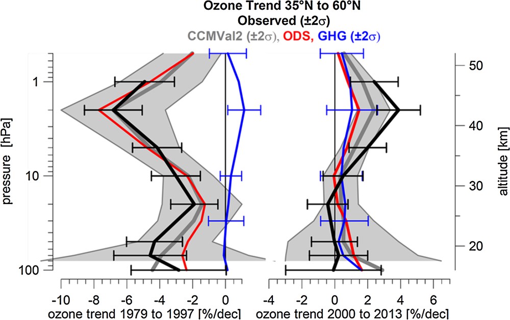
Observed and modelled ozone trend profiles [%/decade] averaged over the 35°N to 60°N latitude band for the periods 1979 to 1997 (left panel) and 2000 to 2013 (right panel). Black line with bars: average of available ground-based and satellite observations, with ±2 standard deviation uncertainty range. Gray line with shading: corresponding mean trends from CCMVal-2 REF-B2 model simulations using ODS and GHG forcing (but only for the subset of seven models that did simulations with fixed GHGs), with uncertainty range given by ±2 standard deviations of individual model trends (not including volcanos and solar cycle). Red line: trend attributed to ODS changes alone from CCM simulations with fixed 1960 GHG concentrations (seven models). Blue line: trend attributed to increasing GHG abundances alone from CCM simulations with fixed 1960 ODS concentrations (nine models). Observed trends are from multi-linear regression accounting for QBO, solar cycle, volcanic aerosol and ENSO. (From Fig. 2-20 from WMO, 2014). Masquer
Observed and modelled ozone trend profiles [%/decade] averaged over the 35°N to 60°N latitude band for the periods 1979 to 1997 (left panel) and 2000 to 2013 (right panel). Black line with bars: average of available ground-based and satellite observations, ... Lire la suite
For the period 2000–2013, observations show a positive trend for mid-latitude upper stratospheric ozone (Fig. 1, right panel, black line), which is captured by the models within the models’ and observational uncertainty (gray line). About half of the simulated ozone increase arises from the ODS decline since 2000 (red line), with the other 50% being contributed by further increasing GHG concentrations (blue line). Hence, rising GHG concentrations act to enhance ozone recovery from ODSs.
While the positive ozone changes since the 2000s in the upper stratosphere are significant and consistent among observations and models, ozone changes in the lower stratosphere are much more uncertain due to a larger variability as well as larger measurement uncertainties, precluding an assessment of significant lower stratospheric ozone trends at the current stage.
2.2 Antarctic and Arctic spring
To derive the contribution of growing GHG abundances to future polar total ozone changes, the new set of CCMI sensitivity simulations is used here. Transient reference simulations driven by observed and best future estimates of ODS and GHG concentrations (i.e. REF-C2) are compared with sensitivity simulations using either fixed ODS (fODS) or fixed GHG (fGHG) distributions of the year 1960. Specifications of the participating CCMs are given in Morgenstern et al. (2017), while the scenarios are explained in Eyring et al. (2013a). The results shown here have been adapted from Dhomse et al. (2018).
Fig. 2 shows the evolution of total column ozone in Antarctic (top) and Arctic (bottom) spring from 1960 to 2100 for the multi-model mean (thick coloured lines), the standard deviation (shaded area) as a measure of model spread, as well as the observational record derived from satellite data. In Antarctica, the reference simulation (REF-C2, red) shows a rapid decline of total column ozone by about one third from 1960 to the end of the 20th century, followed by a gradual recovery over the 21st century. The models do not project a complete return of Antarctic ozone to 1960 values by 2100 consistent with the long lifetime of several ODSs. When the ODS concentrations are kept constant at their 1960 levels over the whole simulation–with otherwise identical REF-C2 conditions–(fODS, brown line), Antarctic spring total column ozone shows only weak year-to-year variations with a small, non-significant positive trend after the middle of the 21st century resulting from stratospheric cooling by rising GHG concentrations. Hence, the temporal evolution of Antarctic spring total column ozone is not strongly influenced by growing GHG concentrations. When GHGs are held constant at their 1960 values but ODSs vary in the same way as in the reference simulation (fGHG, green line), the evolution of total column ozone closely follows that of the REF-C2 reference simulation. Only after the middle of the century, the GHG effect in the REF-C2 simulation slightly accelerates Antarctic ozone recovery and leads to about 10 DU higher total column ozone around 2100. Hence, the evolution of the ODSs exerts the dominant influence on Antarctic total column ozone change, modulated by a minor effect of GHGs in the second half of the century. Although the GHG effect fosters Antarctic ozone recovery from ODSs, the 1960 baseline value will not be reached by the year 2100.

Temporal evolution of multi-model means of total column ozone [TCO, Dobson Units] for Antarctic spring (October, top) and Arctic spring (March, bottom) derived from CCMI scenario calculations for fixed ODSs of the year 1960 (brown), and fixed GHGs of the year 1960 (green), in comparison with a reference simulation including transient ODSs and GHGs of the period 1960 to 2100 (red). SBUV MOD observations are included for the period 1979 to 2017 (black). The solid lines show the multi-model mean; the shaded areas denote ± 1 standard deviation. The dashed line shows the 1960 multi-model mean ozone. (Adapted from Dhomse et al., 2018). Masquer
Temporal evolution of multi-model means of total column ozone [TCO, Dobson Units] for Antarctic spring (October, top) and Arctic spring (March, bottom) derived from CCMI scenario calculations for fixed ODSs of the year 1960 (brown), and fixed GHGs of the ... Lire la suite
In Arctic spring, the evolution of total column ozone is similar to Antarctic spring with a fast decline until the end of the 20th century and a slow recovery afterwards. However, in contrast to southern spring, Arctic spring total column ozone is projected to return to 1960 levels around the 2040s, followed by a continuing growth until the end of the 21st century (‘super-recovery’). When prescribing GHG values for the 1960s (i.e. in SEN-C2-fGHG) throughout the whole projection, total column ozone closely follows the values of the REF-C2 reference simulation until about 2020. Afterwards, it gradually approaches its 1960 values until the end of the 21st century, in contrast to the reference simulation, where the rising GHG abundances induce an additional ozone increase. Hence, as in the Antarctic, the ODSs have been the primary driver of observed Arctic total column trends in the past. However, in contrast to Antarctica, changes in GHGs will exert the dominant control over Arctic ozone distributions by the late 21st century. It is the growth in GHG concentrations that induces a strong increase of Arctic total column ozone, particularly in the second half of the 21st century, as also seen in the simulation without ODS change (senC2fODS, brown line). The GHG effect is a combination of two processes: a reduced chemical ozone depletion in a cooler upper stratosphere and a strengthened Brewer–Dobson circulation (BDC) (e.g., Eyring et al., 2010; Oberländer et al., 2013) leading to a growing poleward and downward transport of ozone in Arctic spring with time. In contrast to the Antarctic, the increasing GHG concentrations are in addition responsible for a strengthening of the dynamical ozone supply of the Arctic stratosphere, which leads to an earlier onset of ozone recovery around the year 2000 and an earlier return to 1960 baseline values.
2.3 Tropics
While growing GHG abundances will accelerate global stratospheric ozone recovery, they have an opposite effect on ozone in the lower tropical stratosphere. Rising sea surface temperatures and tropospheric warming associated with higher GHG concentrations are expected to enhance the dynamical forcing of the stratosphere and lead to an increase in the BDC (e.g., Butchart et al., 2010; Oberländer et al., 2013; SPARC CCMVal, 2010). The BDC describes the mean meridional mass transport in the middle atmosphere. Its main features are upwelling in the tropics, poleward mass transport in the stratosphere and downwelling at higher latitudes (see e.g., Butchart et al., 2010 for a more detailed description). Changes in the BDC directly affect tropical ozone abundances. Fig. 3 (left panel) shows the projected annual zonal mean ozone change between the beginning and the end of the 21st century derived from timeslice simulations with the ECHAM/MESSy Atmospheric Chemistry (EMAC) CCM for the years 2000 and 2095 (Meul et al., 2014). GHG concentrations in the 2095 simulation follow the IPCC SRES-A1b scenario. In the middle and upper stratosphere, a significant global increase in ozone of 10–30% is simulated, as expected from the slowing of chemical ozone destruction in a cooler stratosphere. In the lower stratosphere, however, the increase is confined to the extra-tropical regions with the largest relative changes in the southern polar lowermost stratosphere. In the tropical lower stratosphere, a significant negative ozone change of up to -30% is projected. At the 70 and 50 hPa pressure levels (around 18 to 21 km altitude), the large relative ozone decrease throughout the century is mainly attributed to transport processes (blue bars in Fig. 3, lower and middle right panels), in agreement with other studies (e.g., Oman et al., 2010; SPARC CCMVal, 2010). A significant enhancement of the tropical upwelling in the lower stratosphere between 2000 and 2095 leads to a stronger net export of locally produced ozone molecules. In addition, at 70 hPa, a positive contribution to the ozone change is found from an increased future ozone production (Fig. 3, lower right panel). The more ozone is produced (and the less destroyed) during the transit of the air parcel through the lower stratosphere, the larger the fraction that is transported out of this region within this air parcel. With increasing height, the ozone change attributed to changes in transport becomes smaller and, at 30 hPa, the relative changes due to production and destruction changes dominate (Fig. 3, upper right panel). In summary, while increasing GHG abundances enhance ozone in the tropical upper stratosphere through cooling and reduced chemical destruction, they decrease ozone in the tropical lower stratosphere, predominantly by changes in ozone transport with small contributions from chemical ozone production and destruction.

Change in annual mean zonal mean ozone mixing ratio between the years 2000 and 2095 [ppmv] in simulations with the EMAC chemistry–climate model (left panel; red/blue shading indicates positive/negative changes). Statistically significant changes on the 99% confidence level are coloured. Black contours indicate the relative ozone change [%]. The right panels show the contributions of transport (blue), chemical production (green) and chemical destruction (red) to the ozone change (black) in the tropics (25°S–25°N) at 30 hPa (top), 50 hPa (middle) and 70 hPa (bottom). The grey bars show changes due to nonlinear interactions; white bars show the sum of the individual contributions. (Adapted from Meul et al., 2014). Masquer
Change in annual mean zonal mean ozone mixing ratio between the years 2000 and 2095 [ppmv] in simulations with the EMAC chemistry–climate model (left panel; red/blue shading indicates positive/negative changes). Statistically significant changes on the 99% confidence level are coloured. ... Lire la suite
3 Impact of the climate change scenario
As discussed in the previous sections, the future evolution of ozone is strongly affected by the evolution of future GHG emissions. To assess the potential range of GHG impact on ozone, future projections with climate models and CCMs have been performed using different GHG scenarios. Four Representative Concentration Pathways (RCPs) have been constructed by combining a suite of atmospheric concentration observations and emissions estimates for GHGs through the historical period (1750–2005) with harmonized emissions projected by four different Integrated Assessment Models for 2005–2100 (Meinshausen et al., 2011; van Vuuren et al., 2011). The RCPs differ in the radiative forcing from the respective composition in 2100, ranging between 2.6 W/m2 in the RCP2.6 and 8.5 W/m2 in the strongest RCP8.5 scenario. The RCPs were used to drive the CMIP5 climate model simulations (Taylor et al., 2012) as well as the more recent CCMI model projections (Eyring et al., 2013a). Fig. 4 shows the projected total column ozone (tropospheric plus stratospheric) time series from a subset of CMIP5 simulations (with interactive or offline ozone chemistry) using the four RCP scenarios for GHG concentrations. Also shown is the CCMVal-2 multi-model mean, which is based on the SRES A1B scenario for GHGs (Eyring et al., 2013b; WMO, 2014). Deviations between the two model ensembles exist, which may be due to differences in the models used, the ensemble sizes or the scenarios. Nevertheless, both model ensembles show that, except for the tropics and mid latitudes in the weak RCP2.6 scenario, total column ozone is projected to reach again values of 1980 or higher until the end of the century in all RCP scenarios. The increase in annual mean total column is generally stronger for scenarios with higher GHG abundances and radiative forcings. The weakest sensitivity of total column ozone to the GHG scenario is found in Antarctic spring, where only the RCP8.5 scenario leads to enhanced ozone recovery compared to the other RCPs. In the tropics, no recovery of total column ozone is projected in the CMIP5 models for the three moderate scenarios or by the CCMval models. Using the EMAC CCM with full tropospheric and stratospheric chemistry, Meul et al. (2016) showed that in the tropics, the upper stratospheric ozone column will recover due to the decline in ODSs and the GHG-induced stratospheric cooling. This recovery is most pronounced in the RCP8.5 scenario. It is overcompensated by a decrease in the lower stratospheric ozone column, which again is most pronounced in the RCP8.5 scenario, where the increase in the BDC is strongest. In addition, there is a growing and scenario-dependent role of tropospheric ozone. The RCP8.5 scenario projects a strong growth of CH4 concentrations in the second half of the 21st century. This will result in enhanced tropospheric ozone production, thus mitigating the remaining loss in tropical total column ozone around 2100. Hence, in the tropics future total column ozone will be the product of partly counteracting processes in the upper stratosphere, lower stratosphere and troposphere (see also Shepherd et al., 2014).

The 1980 baseline-adjusted total column ozone time series from 1960 to 2100 for the CMIP5 multimodel mean with interactive chemistry (coloured lines) and the CCMVal-2 multimodel mean ozone database (black line) for different regions. All time series by construction go through 0 in 1980. The RCP2.6, RCP4.5, RCP6.0, and RCP8.5 are shown in blue, light blue, orange, and red, respectively. The corresponding color-coded stippled areas show the 95% confidence interval of the CHEM multimodel mean simulations. (From figures 2-23 and 3-17 in WMO, 2014; derived from Eyring et al., 2013b). Masquer
The 1980 baseline-adjusted total column ozone time series from 1960 to 2100 for the CMIP5 multimodel mean with interactive chemistry (coloured lines) and the CCMVal-2 multimodel mean ozone database (black line) for different regions. All time series by construction go ... Lire la suite
4 Relevance of nitrous oxide and methane
Nitrous oxide (N2O) and methane (CH4) are both GHGs that directly affect ozone as they are key source gases for the NOx and HOx chemical ozone loss cycles. With reduced future halogen levels, the NOx loss cycle will dominate chemical ozone destruction in the upper stratosphere, while the HOx loss cycle will dominate in the lower stratosphere and in the mesosphere. The future burden of N2O and CH4 in the stratosphere will be different depending on the RCP. Revell et al. (2012) investigated the sensitivity of future ozone to changes in N2O and CH4 by performing CCM simulations in which either N2O or CH4 concentrations were prescribed according to the RCP2.6 (with lower N2O/CH4 increase) and RCP8.5 (with strongest growth of the two substances) scenarios, while the other GHG abundances followed the SRES-A1b scenario (Fig. 5). In the middle stratosphere, ozone will be substantially lower by the end of the 21st century if N2O increases according to the RCP8.5, as more NOx will be produced and more ozone chemically destroyed (Fig. 5, top). In the lower tropical stratosphere, there will be more ozone, partly due to enhanced UV availability (‘self-healing’ effect of ozone deficit higher up) and partly due to enhanced chemical production associated with CH4 oxidation caused in the troposphere by the higher NOx concentrations in the RCP8.5 scenario. The response of ozone to higher CH4 concentrations in the RCP8.5 scenario arises from a combination of direct and indirect effects (Fig. 5, bottom). In the mesosphere, more CH4 in the RCP8.5 scenario will lead to more HOx which chemically reduces ozone. Below 45 km, more CH4 leads to more ozone via a combination of different mechanisms involving deactivation of chlorine, ‘smog’ photochemistry, and slowed ozone loss rates due to cooling from enhanced H2O after CH4 oxidation. More details are given in WMO (2014).
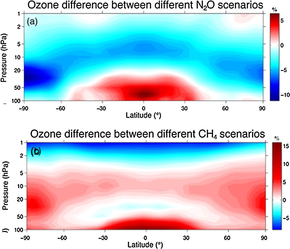
Ozone changes in the 2090s due to different N2O and CH4 scenarios, computed with the National Institute of Water and Atmospheric research (NIWA)-SOCOL chemistry–climate model. (a) Difference between ozone in the 2090s under the N2O–RCP8.5 scenario and ozone under the N2O–RCP2.6 scenario [in percentage of N2O–RCP2.6 ozone], (b) same but for CH4-RCP8.5 ozone minus CH4–RCP2.6 ozone in the 2090s. (Adapted from figures 2-25 in WMO (2014) and Revell et al., 2012).
Acknowledgements
This work has been supported by the Deutsche Forschungsgemeinschaft (DFG) within the DFG Research Unit FOR 1095 “Stratospheric Change and its Role for Climate Prediction” (SHARP). The author is grateful to Sandip Dhomse and the CCMI modellers for providing Fig. 2.