

1 Introduction
Sea level variation reconstruction related to climatic changes are carried out using numerous tools allowing direct reading of the paleo-levels recorded by the beach rocks, the marine terraces, the coral reefs or by the evaluation of the variations of the ice volumes through the foraminifer oxygen isotopes and submerged speleothem in coastal areas (Antonioli et al., 2001; Bard et al., 1996; Chappell, 2002; Cutler et al., 2003; Rohling et al., 2009; Siddall et al., 2003). Those allowed quantifying the amplitudes related to sea level variations.
Qualitative and quantitative methods based on the microfauna assemblage distributions allowing the reconstruction of the paleo-depths are also used to characterize sea level fluctuations (Hayward, 2004; Hohenegger, 2005; Milker et al., 2011; Morigi et al., 2005; Rossi and Horton, 2009; Spezzaferri and Tamburini, 2007). These methods are based on a very good knowledge of the distribution of living foraminifera and on the assumption that the ecological requirements of specific taxa have not changed over time. In this study, we use this principle to establish a transfer function in which the recent benthic foraminifer assemblages of the East-Corsican margin are used for modelling the depths according to the formula: Hm,j = ac,0 + Zj,k·ac,k, where Hm,j is the modelled depth at each site j, Zj,k is the matrix containing the values of the principal components used in the model. Each line (j) is associated with a site; each column k is associated with an used principal component. Both the scalar ac,0 and the vector ac,k are estimated by calibration based on least-squares interpolation.
The level of correlation observed between these modelled depths and the actual depths will allow the application of this equation to fossil benthic foraminifer assemblages. Comparison with other eustatic curves will allow discussing this method of sea level reconstruction and evaluating the difficulties of using benthic assemblages as tools of variations in the water column.
2 Study area
Located in the northern part of the Tyrrhenian Sea (Western Mediterranean), the East-Corsica margin is a continental shelf region varying from 5 to 10 km in width in the northern part to 25 km in the southern one. The continental shelf characterizing the East-Corsica margin is narrow, with a shelf break situated around 110–120 m (Gervais, 2002; Gervais et al., 2004). This continental shelf is followed by a steep continental slope incised by numerous meandering canyons (Gervais, 2002). The latter open out into a deep basin, which is characterized by a depression named Corsican Trough.
3 Materials and methods
3.1 Micropaleontological and stable isotope analyses
Before performing micropaleontological analyses, samples were washed and sieved (63 μm) on the sedimentary fraction > 150 μm. The recent benthic foraminifers of the East-Corsica basin were studied in 45 surface samples from the interface cores collected at depths ranging from 7 to 868 m, and 101 benthic foraminifer taxa were identified (Angue Minto’o et al., 2013). The identification of 84 taxa of fossil benthic foraminifer was possible via the analysis of 291 samples from the GDEC-4 borehole drilled at a water depth of 492 m in the East-Corsica margin covering the last 550,000 years (Angue Minto’o et al., 2016).
Oxygen stable isotope measurements were performed on specimens of planktonic foraminifera species Globigerina bulloides and G. ruber (white) from the 250–315 μm size fraction, Neogloboquadrina pachyderma (dextral) from the 200–250 μm size fraction, and on the epifaunal benthic foraminifera Cibicides wuellerstorfi, Cibicidoides pachyderma and Cibicidoides kullenbergi found in the > 150 μm size fraction (Toucanne et al., 2015).
3.2 Species selection and principal component analysis
In this study, MatLab generic functions are used for the computations. We call M0(i,j), the initial matrix of species to be consider in the analysis. M0(i,j) consists of relative abundances of the all benthic foraminifers (101 species) identified in the surface samples, where i is the site and j the species. With the aim of obtaining qualitative results, the reduction of the number of species of M0(i,j) is made by eliminating species with a median equal to 0. Because Principal Component Analysis (PCA) is based on correlation analysis and hence variation quantifications, consequently, on 101 recent benthic foraminifer taxa identified, only 33 taxa were retained and are listed in Table 1. For these 33 species, the relative abundance, at one site, is always calculated using the total number of individuals per site based on the 101 species. This allowed maintaining independence between the frequencies retained, i.e. the sum of the species frequencies per site does not equal 1, and the dependent and untreated variable is “the other species”
Presentation of the 33 benthic foraminifers derived from the analysis of the interface samples and having a median greater than 0. These 33 taxa were selected for the principal component analysis.
| Retained species | Order number |
| Amphicoryna scalaris | 1 |
| Bulimina marginata | 2 |
| Bulimina costata | 3 |
| Bigenerina nodosaria | 4 |
| Biloculinella labiata | 5 |
| Bolivina spathulata | 6 |
| Cibicides wuellerstorfi | 7 |
| Cibicides lobatulus | 8 |
| Cibicides sp. | 9 |
| Cyclogyra carinata | 10 |
| Cassidulina carinata | 11 |
| Cassidulina crassa | 12 |
| Cassidulina minuta | 13 |
| Elphidium macelum | 14 |
| Fissurina cucullata | 15 |
| Gyroidina orbicularis | 16 |
| Gyroidina altiformis | 17 |
| Hoeglundina elegans | 18 |
| Hyalinea balthica | 19 |
| Lenticulina sp. | 20 |
| Melonis barleeanus | 21 |
| Pseudoclavulina crustata | 22 |
| Quinqueloculina duthiersi | 23 |
| Quinqueloculina viennensis | 24 |
| Quinqueloculina seminulum | 25 |
| Rosalina globularis | 26 |
| Spiroloculina escavata | 27 |
| Sigmoilopsis schlumbergeri | 28 |
| Spiroplectinella sagitula | 29 |
| Textularia agglutinans | 30 |
| Textularia truncata | 31 |
| Valvulinaria bradyana | 32 |
| Uvigerina mediterranea | 33 |
PCA is based on the covariance matrix (Mc) estimated on the basis of the species abundance matrix by site:
The eigenvalues and eigenvectors of the matrix Mc are computed to establish, respectively, the weight (variance) associated with each component and the coefficients of the principal components. Thus, the matrix of the eigenvectors Cjk, and the coefficients of the principal components are calculated as well as the diagonal matrix of the eigenvalues Djk. The new matrix Cjk verifies the following equality:
The principal components are obtained by a “rotation” of the assembly matrix (Mij) along the principal vectors described by the matrix of eigenvectors or coefficients of the components
It is important to keep in mind that the matrix Zik contains the same amount of information as the initial abundance matrix Mij from which Zik has been derived. The information is organised in a new way, the components being independent of one another. Hence, at each site i, Zik provides the local value of component k, while Mij provides the local abundance of species j, the number of species and of components being the same (33).
The matrix Cjk co-relates the principal components and the species. Even if it is computed from the data, it contains an estimation of a relation that is supposed to be valid for any assemblage (not only the ones in the data). Cjk is the same for all sites (observed or noted) and is the base of the generalization.
At each new site,
We can evaluate the possibility of obtaining a model linking the species assemblages and the depth of the sites.
3.3 One-component models
For each component Zk, one can define a depth model Hk obtained by linear regression for the depth H:
3.4 Multi-component models
For models consisting of several components, the method applied is the same. A depth model is obtained by linear regression using the least squares method. Here the most representative component of the variance is used. Thus, a depth model Hn can be defined, where n is the number of components used (from the highest to the lowest):
The performance of the model Hn can be associated with the An function,
The value A6 will give the correlation level of a regression model based on the six most important components in terms of assemblage variability.
3.5 Determination of the freedom factor
A freedom factor (λn) of a model consisting of principal components n with respect to the points number (P) of calibration/validation is defined by the following formula:
A freedom factor is defined to quantify the robustness of the models based on the number of its number of freedom degrees. For a model based on n principal components, its freedom factor (Ln) is quantified by the number of data points used for calibration (P) and the number of degrees of freedom of the used model (n + 1, if n PCs are used).
If this factor is close to the unit, the model is robust in terms of degrees of freedom. If the factor is close to zero, the model is not robust, and there are too many degrees of freedom compared to the size of the data available and the basis of its construction. In our study, P = 44.
An performance indicator of the model could be defined as the “good” compromise between the correlation level and its performance or factor of freedom. The quality of a model Hn described by the function Qn is defined as follows:
3.6 Calibration and validation of the models
After a ranking based on their depths, the 44 sites are divided into two groups. The first one is composed of one site out of two and it is called “calibration”. This group includes variables with an index c. The second group consists of the other sites and it is called “validation”. This validation group is characterized by variables with an index v. The coefficients ak are calculated by regression on the basis of the following system of equations:
The modelled values will then be:
The calibration coefficients are then used for the validation data in order to obtain the simulated data Hm,v:
4 Results and discussion
4.1 Principal component analysis (PCA)
The results of the PCA show that a very important part of the variance (> 90%) is contained in the first five eigenvalues, or principal components (Fig. 1). The contribution of each species to the two main components can be visualized by the respective contributions of each species (Fig. 2). It may be noted in Fig. 2 that the species that contribute the most to the expression of the first component are M. barleeanus (21) and U. mediterranea (33). This component is modulated (attenuated) by the presence of C. carinata (11), R. globularis (26), and Q. duthiersi (23). The second component, however, is expressed by the “competition” between C. carinata and R. globularis (Fig. 2).
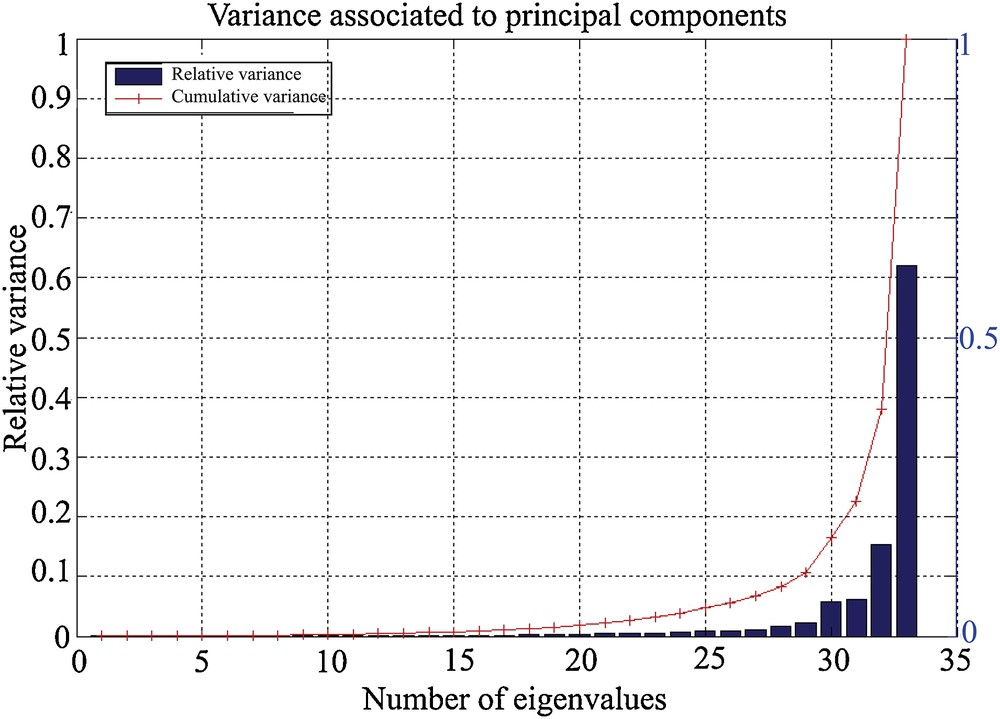
Variance associated with the 33 main components. The majority of the variance is contained in the first five eigenvalues, or principal components.
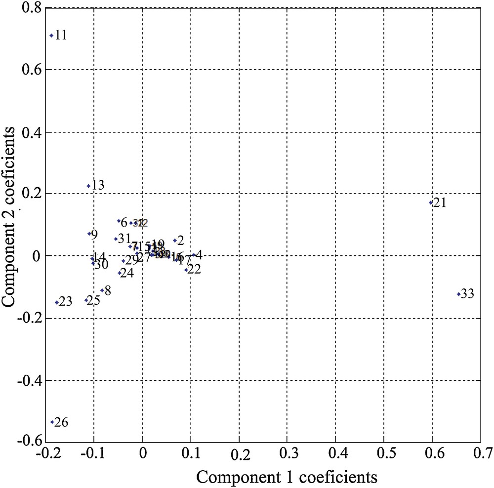
Species contribution to the two main components.
4.2 Correlation between depths and principal components
The correlation levels between the depth of the sites and the principal components associated with the assemblages are presented in Fig. 3. The function B is represented by the blue bars that indicate the correlation level of each component with the depth. The function A is represented by the red curve. This latter indicates the correlation level reached by regression between a set of N components and the depth. Thus, the component 33, which is the first in importance, is the one that shows the best correlation with the depth. This component alone allows having a correlation level higher than 95% (Fig. 3). The other components are individually weaker. However, they allow increasing the total correlation to more than 99% if all 33 components are used to reproduce the 44 depths.
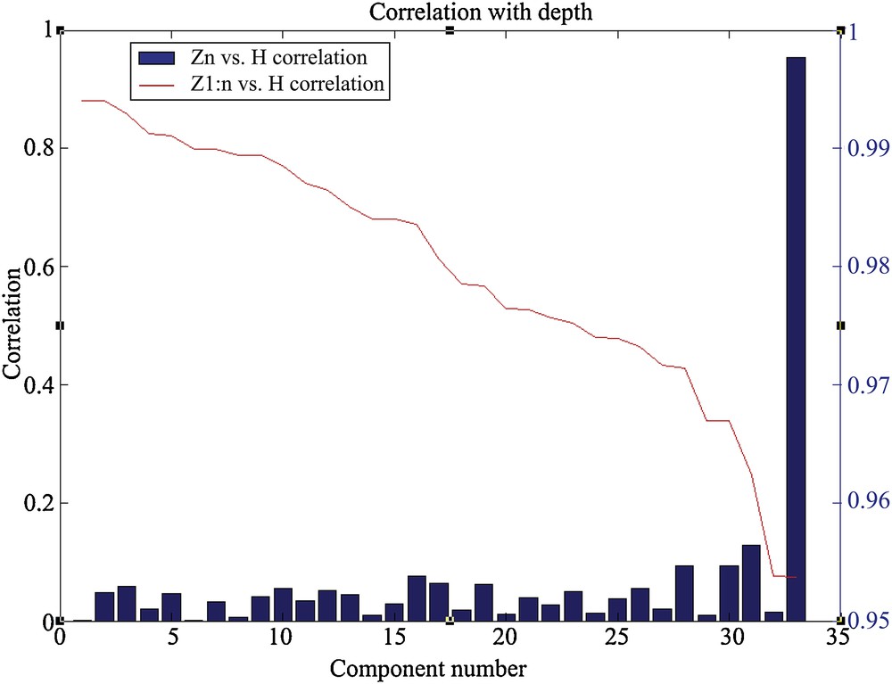
Correlation between the depth of the sites and the principal components. The blue bars represent the function B and the red curve characterizes the function A.
The best model is not necessarily the one that allows obtaining the best correlation between true values and model values estimated on these same true values. The number of degrees of freedom associated with the calibrated models and the number of validation points must be taken into account, because the models are calibrated on the validation points. Thus, all models Hk have two degrees of freedom: the coefficients a and b. The models Hn have n + 1 degrees of freedom. By absurdity, a model whose number of degrees of freedom is equal to the number of calibration/validation points will always present a correlation of 100%.
The representation of the function Qn (Fig. 4) shows that the use of a small number of components can be advantageous in terms of robustness of the chosen model.
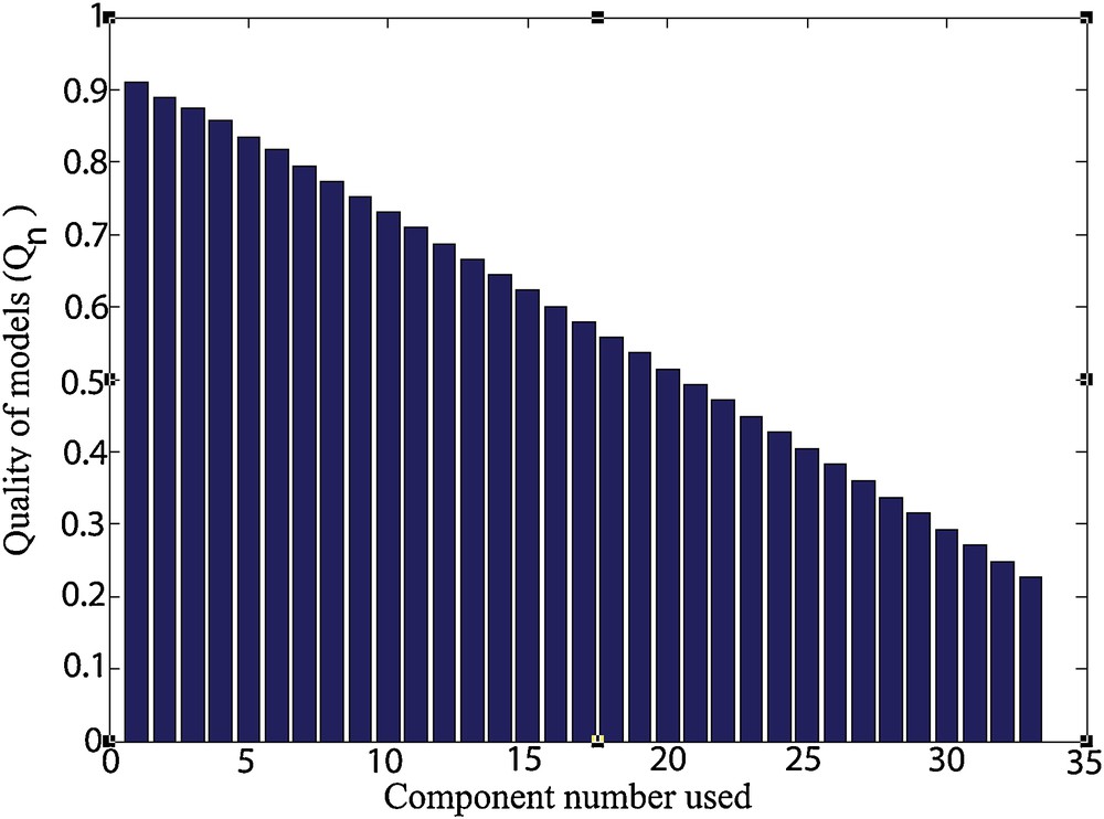
Representation of the function Qn.
4.3 Evaluation of the models
The evaluation is made for models built with a number of variable components (between 1 and 6). The model with all the data (blue curve) serves as a reference (Fig. 5). Calibration 1 (cal 1) and validation 1 (val 1) are obtained as described in the paragraph related to calibration and validation of models: the first set is for calibration and the second set for validation. The models cal. 2 and val. 2 are obtained by reversing the use of the sets (Fig. 5).
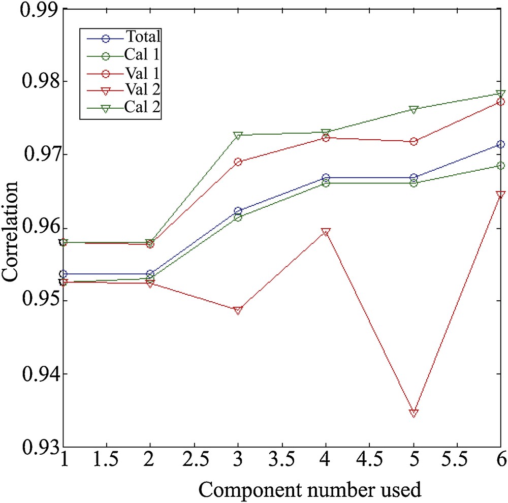
Evaluation of the different models: the one with all the data (blue curve) and the models calibration (green curves) and validation (orange curves).
For cal. and val. 1, we obtain a calibration model that is slightly less efficient than the reference one, while the validation is generally better (Fig. 5). This means that the validation set is closer, in terms of assemblages, to what can be explained by the depth. Overall, the correlation improves with the number of components used. This improvement is increasing for the reference and for the calibration (Fig. 5). For the validation model, the two minor contribution components (2 and 5) reduce the performance of the model. When we reverse the use of sets, we fall back on a reverse result, and more “classic”. Calibration, done on less data than the reference, is more efficient (but with a lower freedom factor); validation is less well than calibration and reference.
The choice seems to be made between 1, 4, or 6 components, even if it remains conceivable to use only the useful components. Correlations are performance indicators. It is therefore important to visualize the correlations presented in Figs. 6 and 7, in which a loss of linearity can be observed from 700 m depth with the error margins of 43 m and thus 86 m in 2σ.
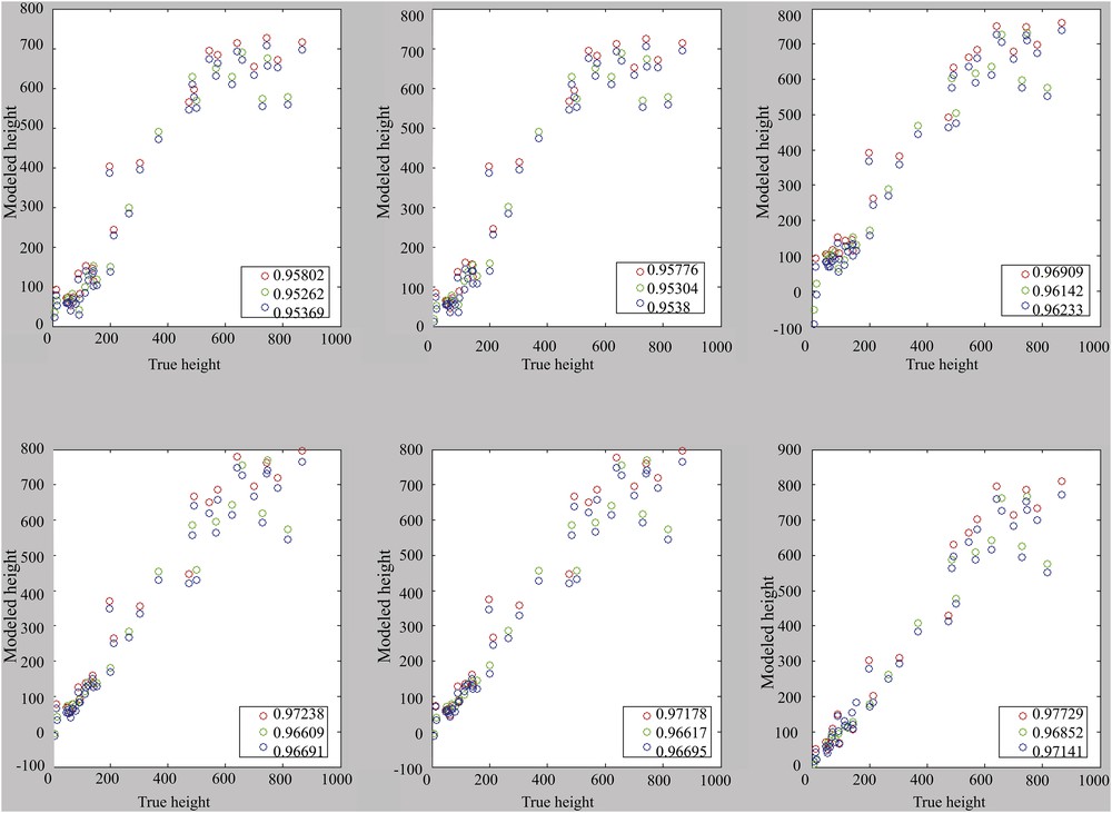
Correlation for models with the use of one to six main components (from top left to bottom right). Calibration set: cal. 1. Reference (blue), calibration (green), and validation (red).
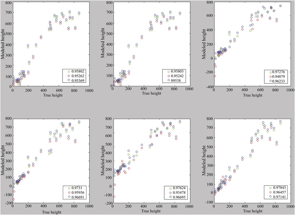
Correlation for models with the use of one to six main components (from top left to bottom right). Calibration set: cal. 2. Reference (blue), calibration (green) and validation (red).
4.4 Choice of the final model
Principal component analysis allows us to “focus” the variance of the assemblages on a very small number of variables (components), which is very useful in order to reduce the number of freedom degrees of the models obtained by regression.
Out of 33 components (as much as the selected species), we will keep four components (28, 30, 31 and 33), which means that the regression model is based on the estimation of five parameters.
The model obtained made it possible to have a 97.13% correlation on all the sites. The calibrated model on 22 sites (performance of 96.85% in self-application) displays a correlation of 97.72% on the validation set. The performance of the chosen model is illustrated in the Fig. 8.

Performance of the selected model: correlation between “true” depths and modelled depths.
4.5 The structure of the model
The structure of the model is presented in Fig. 9. It can be noted that the final contribution to explaining the depth variability is very distinct from the distribution of the coefficients associated with each species. This is because the relative abundance of each species has not been standardized. Thus, there are two species that contribute significantly: M. barleeanus and U. mediterranea. M. barleeanus explains the variations of depth at shallow depths and U. mediterranea explains the depth beyond 100 m.

Model structure: coefficients and variance per species.
4.6 Application of the model and comparison with the semi-quantitative method
4.6.1 Numerical model
The application of the model H(i) = 109.6103 + C1 × F1(i) + C2 × F2(i) + … + C33 × F33(i) (where Ci corresponds to the coefficient of species i and Fi to its frequency) on fossil benthic foraminifers species allowed us to obtain the curve of paleo-depths variation. The reconstructed paleo-depths range from 622 ± 86 m to 21 ± 86 m. In general, the variation of these paleo-depths correlates quite well with the variations of the sea level (Fig. 10). A global trend marked by an increase in depth during periods of high sea level is observed. Interglacials are characterized by the removal (or melting) of glaciers that conduct to an increase in sea level (Dorale et al., 2010) and therefore to an increase in the water level above the seabed. This could justify this rise of the paleo-depths during these warm climatic periods. However, these paleo-depth variations are characterized by very large amplitudes.
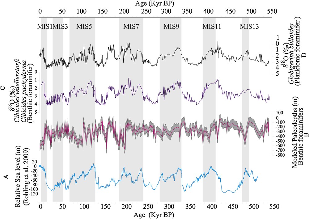
Characterization of the paleo-depth variation during the last 500,000 years. Comparison between: A, the relative sea level variation curve (Rohling et al., 2009); B, the curve of variation of the modelled paleo-depths; C and D, curves of changes in oxygen isotopic ratio of benthic (Cibicides wuellerstofi and Cibicides pachyderma) and planktonic (Globigerina bulloides) foraminifers.
Based on the fact that these modelled amplitudes are affected by (1) local effects related to the morphology of the basin, which is shallow and semi-marine (close to the sources), (2) changes in trophic conditions at the bottom strongly influencing the variations of benthic microfauna assemblages, (3) uncertainties related to the calculation method and the bathymetry. Normalization from 0 to 120 m was thus made on the values of paleo-depths and the sea level variation curve obtained was compared with the eustatic curve established by Rohling et al. (2009) and smoothed in the same way (Fig. 11). This results in a fairly good correlation between these two curves.

Standardized and smoothed sea level variation curve compared with the smoothed sea level variation curve from Rohling et al. (2009) and the relative abundance variation of benthic foraminifers Melonis barleeanus and Uvigerina mediterranea. A good correlation is observed between normalized eustatic variations and abundance variations of Melonis barleeanus/Uvigerina mediterranea. A significant shift during periods of high sea level is observed between the two eustatic curves.
However, very large temporal offsets in amplitude and in time are observed between the two interglacial curves: between 290 and 280,000 years (15 ka), 200 and 180,000 years (15 ka), 170 and 160,000 years (15 ka), 125 and 100,000 years (30 ka) and between 60 and 30,000 years (30 ka, Fig. 11).
These offsets therefore appear during periods of high sea level that are globally characterized by a decrease in the organic matter inputs related to the theoretical distance of the sources (Cortina et al., 2013) and by a decrease in the ventilation at the sea bottom (Toucanne et al., 2012). The offsets result from an underestimation of the depths that could be related to the non-integration in the model of the changes in bottom trophic conditions strongly influencing the variations of benthos foraminifer assemblages (De Rijk et al., 2000; Fontanier et al., 2002; Gooday, 2003; Jorissen et al., 1995; Mackensen et al., 1990; Murray, 1991; Schönfeld, 2002a; Schönfeld, 2002b). Indeed, U. mediterranea and M. barleeanus are the two species of benthic foraminifers that strongly influence the calculation of paleo-depth. This is illustrated by the perfect correlation between the normalized eustatic variation curve and the variation in their cumulative abundance curve (Fig. 11). U. mediterranea and M. barleeanus are species related not only to the quality but also to the intensity of organic matter inputs to the bottom. M. barleeanus is known as a species that develops in environments where there is the refractory organic matter (Fontanier et al., 2002; Lutze and Coulbourn, 1984) and U. mediterranea adapts to environments with moderate fluxes of labile organic matter (Lutze and Coulbourn, 1984; Schmiedl et al., 2000).
Based on this low correlation and the error margins obtained (± 86 m), and on the significant offsets observed with the relative sea level variation curve (15 and 30 ka), we can say that on a time scale of 100,000 years, the method is difficult to apply. Because at this time scale, the variation amplitudes of the sea level (the order of one hundred meters) remain lower compared to the margin of error (± 86 m) applied to our model. The transfer function could therefore be more suitable on a million-year time scale in which sea level variations are recorded with larger amplitudes and where isotopes are difficult to use.
5 Conclusion
Depth modelling using 33 species of recent benthic foraminifers in the East Corsica margin was based on a principal component analysis (PCA) that allows us to obtain the model H(i) = 109.6103 + C1 × F1(i) + C2 × F2(i) + … + C33 × F33(i) with a correlation of 97.1%. The application of this model on fossil benthic foraminifers conducts to the establishment of a paleo-depth variation curve with a margin of error of ± 86 m. The resulting sea-level variation curve shows significant shifts during high sea levels, which could partly be explained by the significant evolution of trophic conditions during interglacial periods. This margin of error and this offset can be indicators of the limit of application of this transfer function on a scale of 100,000 years where the sea level variation amplitudes are in the order of a hundred meters. On the other hand, on a million-year scale that is characterized by variation with larger amplitudes, this model could provide an interesting estimation. In order to reduce the margin of error and to avoid a significant signal disturbance, it is necessary to take into account, in the function of transfer, the environmental parameters, in particular the concentration and quality of the organic matter and other nutrients that largely affect the bathymetric distribution of benthic foraminifers.
This paper is invited in the frame of the 2017 Prizes of the French Academy of Sciences (“bourse Louis-Gentil de l’Académie des sciences”). Il has been reviewed by Philippe Janvier, Dominique Gibert, and Vincent Courtillot.
Supplementary data associated with this article can be found, in the online version, at https://doi.org.10.1016/j.crte.2018.09.003.