


 CC-BY 4.0
1. Introduction
In sedimentary basins, the impedance contrast at the interface between soft sedimentary layers and the underlying bedrock leads to the trapping of seismic waves within the sedimentary in-filling. This gives rise to complex wave phenomena (body wave resonance, generation and diffraction of surface waves at the edges of the basin, vertical and lateral reverberations, focusing effects) which highly depend on the three-dimensional (3D) geometry of the basin and often result in an increased amplitude (or “amplification”) and duration of the ground motion (or “duration lengthening”). This modification of ground motion due to local geology is referred to as site effects. Site effects have been the subject of many studies, especially since the devastating 1985 Mexico earthquake that brought to light the influence of local soil conditions on the strong amplification of ground motion observed in Mexico City, despite the long distance to the seismic source [e.g., Campillo et al., 1989]. This example, along with many other observations around the world [e.g., Kawase, 1996, Graves et al., 1998, Lebrun et al., 2001, Roten et al., 2008, Bindi et al., 2011, Ktenidou et al., 2016], makes it clear that the quantification of these site effects is essential for seismic hazard assessment (SHA). Because they are related to local soil conditions, site effects can be highly variable from one site to another, and therefore require site-specific studies for a robust estimation that accounts for the whole complexity of wave phenomena, in particular in 3D geological structures.
The French-German DARE project (Dense ARray for site effect Estimation) has been conceived and designed in this line. The idea is to implement various and complementary approaches to perform a detailed study of site effects at a target site located in the French Rhône valley. The area hosts critical facilities including nuclear installations, thereby motivating the need for robust SHA studies locally. This site is located on the deep and elongated Messinian Rhône Canyon, whose geometry and lithological characteristics make it a good candidate for generating multidimensional site effects. DARE is centred on the exploitation of dense and complementary datasets acquired in the area [Froment et al., 2022b]. The project proposes to investigate the interest of using such datasets for a robust estimation of site effects, especially in low-to-moderate seismicity areas such as metropolitan France.
One first, standard approach considered in DARE relies on earthquake recordings through the calculation of so-called site/reference Standard Spectral Ratios [SSR, Borcherdt, 1970]. SSR estimate the local seismic amplification by direct comparison between earthquake seismograms simultaneously recorded at a given site station laying on a sedimentary basin (subject to site effects) with respect to a nearby reference station (typically on a bedrock outcrop, considered free of site effects). This empirical method has proven to be efficient for a robust quantification of site effects in various configurations. The implementation of this method may however show some difficulties in low-to-moderate seismicity areas, such as mainland France [Traversa et al., 2020], where moderate to large earthquakes (Mw > 5.0) have long return periods, therefore requiring long deployments. Alternative approaches may thus be considered to complement such seismicity-based analysis of site effects. To this end, the DARE project investigates two main research tracks in order to explore the potential of using weak but ubiquitous vibrations—known as ambient seismic noise—as an alternative source of data for estimating site effects due to complex wave propagation in sedimentary basins [e.g., Boué et al., 2016]. On one hand, seismic noise can be used directly for empirical estimations of site effects, via H/V analysis [e.g., Bonnefoy-Claudet et al., 2006, Spica et al., 2017, van Ginkel et al., 2019] or noise-based SSR estimations [e.g., Perron et al., 2018, Gisselbrecht et al., 2023]. On the other hand, ambient noise could also be used in a more indirect way as the initial ingredient to build seismic models of the target site that could then be used for numerical prediction of the ground motion and thus of seismic amplification. The present paper focuses on this numerical aspect.
By giving access to the complete wavefield, simulations help to evaluate the spatial variability of site effects and more importantly to understand the underlying physical parameters to which they are sensitive [e.g., De Martin et al., 2021]. 1D modelling of body-wave resonance phenomena is a first way to calculate the response of a sedimentary layer overlaying a rigid bedrock [e.g., Thomson, 1950, Haskell, 1953]. However, in the presence of complex geological structures, several studies have shown the limitation of 1D numerical simulations, and the necessity of 2D or 3D simulations of seismic wave propagation to reproduce the observed amplifications [e.g., Kawase, 1996, Smerzini et al., 2011, Matsushima et al., 2014, Ktenidou et al., 2016]. Gélis et al. [2022] reach the same conclusions for our target site, as they observe that 1D simulations do not reproduce the amplification measured in the Tricastin basin, in particular regarding its maximum amplitude (up to a factor 8) and its broadband spectral character, typical of 3D wave propagation effects [Chávez-García et al., 2000, Cornou and Bard, 2003, Bindi et al., 2009, Michel et al., 2014]. The conclusions of this previous study by Gélis et al. [2022] form the motivation for the use of 3D numerical simulations in our work. 3D simulations have become more affordable lately thanks to the rapid increase of computational resources and to the development of dedicated software, using in particular spectral-element methods [SEM, e.g., Komatitsch and Vilotte, 1998, De Martin, 2011, Trinh et al., 2019]. These developments led to many applications, notably in sedimentary basins with complex geometries that require detailed simulations [e.g., Komatitsch et al., 2004, Maufroy et al., 2015, 2016, Chaljub et al., 2010, 2015, Paolucci et al., 2015, Thompson et al., 2020, De Martin et al., 2021, Panzera et al., 2022]. These simulations however require an accurate knowledge of the subsurface, both in terms of geometry and of seismic properties (S-wavevelocity VS, P-wave velocity VP, density 𝜌, and S- and P-wave attenuation factors QS and QP). As a consequence, these numerical approaches also rely on field data and geophysical surveys in order to constrain numerical models and define reliable input parameters for the simulations. On the other hand, seismic data (earthquake and noise recordings) are also essential to provide observations which the outputs of the simulations can be compared and calibrated with.
Most studies involving 3D numerical simulations for site effect estimation rely on layered models [e.g., Taborda and Bielak, 2013, Maufroy et al., 2016, De Martin et al., 2021, Panzera et al., 2022]. In these models, layers are separated by interfaces associated to sharp impedance contrasts, and seismic properties are usually assumed either homogeneous or varying only vertically within each layer. The geometry of the interfaces is often derived from geological knowledge (borehole data, field campaigns, surface mapping or interpreted cross-sections), from the interpretation of active seismic migrated images, or from H/V spectral ratio analysis, while seismic properties are often estimated from a limited number of local measurements such as Ambient Vibration Analysis (AVA) and extrapolated to the entire layers, assuming vertical but no lateral variations within the layers [e.g., Manakou et al., 2010, Molinari et al., 2015, Cushing et al., 2020, Panzera et al., 2022].
In the present paper, we propose an alternative approach that uses ambient-noise surface-wave tomography (ANSWT) for building 3D seismic models of the target area. ANSWT is a tomographic method that has proven very successful for imaging shear-wave velocities (VS) at the crustal and lithospheric scales [e.g., Shapiro et al., 2005] and more recently at smaller, basin scales [e.g., Boué et al., 2016, Chmiel et al., 2019]. Taking full advantage of the deployment of dense seismic networks, this passive seismic imaging technique is particularly attractive. ANSWT has the advantage to provide a quantitative model of shear-wave velocity structure in 3D, including both vertical and lateral variations, at relatively low cost. However, ANSWT provides smoother models compared to active seismics and to the geology-based layered models usually considered in numerical simulations. The aim of this paper is to investigate the use of standard ANSWT models for the numerical estimation of seismic amplification and for site effect assessment. More precisely, the question we address here is the following: what are the potential and limitations of 3D numerical simulations based on standard ANSWT models to assess seismic amplification in complex sedimentary basins?
The paper is organized as follows. Section 2 presents the target zone, its geological context, and the seismic data acquired in the frame of the DARE project. Section 3 reminds the steps of the standard ANSWT workflow used to build a 3D VS model of the target site, and explains how we derive other seismic properties (VP, 𝜌, QS, QP) in order to build a full 3D seismic model. In Section 4, we present our numerical results and the seismic amplification predicted in the 3D model, which we compare with observed, earthquake-based SSR, as well as with noise-based SSRn and with 1D approximations. Finally, we discuss the results in Section 6, highlighting the potential of using ANSWT models for the seismic characterization of sedimentary basins, but also underlining some limitations in their use for the numerical estimation of site effects, which leads us to propose perspectives for future work.
2. Target site and data
The DARE project targets the area of the Tricastin Nuclear Site (TNS) in the French Rhône Valley (Figure 1). The TNS is located on the Messinian Rhône canyon that was dug about 6 million years ago during the Messinian Salinity Crisis (MSC) by the paleo-Rhône river in older geological formations. In this area, the geological basement is mainly constituted by hard and thick (several hundreds of meters) lower Cretaceous limestones (Barremian), so-called “Urgonian” limestones, which we consider to be the reference bedrock unit in the region. These Urgonian limestones are overlain by more detrital lower to upper Cretaceous (Aptian to Turonian) formations (sands, sandstones, and marls), and then by Tertiary marine and continental detrital formations. These units are called hereafter “post-Urgonian Cretaceous (and/or Tertiary) formations” in order to distinguish them both from the Urgonian bedrock and from post-Messinian sediments. Indeed, after the MSC, the canyon has been filled with Pliocene sediments of marine (sands and clays) and continental (fluviatile conglomerates) origins, nowadays covered by the Rhône lower-to-recent Quaternary terraces. In 2019, when the DARE project was initiated, the local geology of the Messinian canyon remained poorly documented in the region of Tricastin. Gélis et al. [2022] provide some first insights about the canyon rims and the local subsurface characteristics based on borehole data, geological study, and local 1D geophysical characterization campaigns (H/V and AVA measurements). This first study provided local knowledge about the characteristics (thickness and VS velocities) of the sedimentary canyon in-filling and of the underlying bedrock at two sites in the area. A first site is located 2–3 km south of the TNS (seismic station E1/BOLL in Figure 1), on top of the sedimentary basin. At this site, Gélis et al. [2022] show that the base of the canyon reaches a depth of at least 500 m, incising—or, at least, lying directly on top of—high-velocity Urgonian limestones. The 2nd site is station G6/ADHE on a nearby outcrop of Urgonian limestones, which Gélis et al. [2022] characterize as a hard rock site with an estimated VS30 (the average shear-wave velocity in the first 30 m) of about 2000 m/s. At larger depth, the 1D VS profiles show velocity rapidly increasing with depth and reaching about 3000 m/s beyond 50 m depth. Gélis et al. [2022] present the various criteria for considering G6/ADHE as a good reference for SSR calculations. It is worth noting that VS profiles obtained at ADHE and BOLL are consistent (i) with available geological data [e.g., Bagayoko, 2021, Do Couto et al., 2024] and (ii) with each other in terms of mean velocities at depth, therefore giving a reference velocity of VS ≅ 3000 m/s for the deep Urgonian substratum.
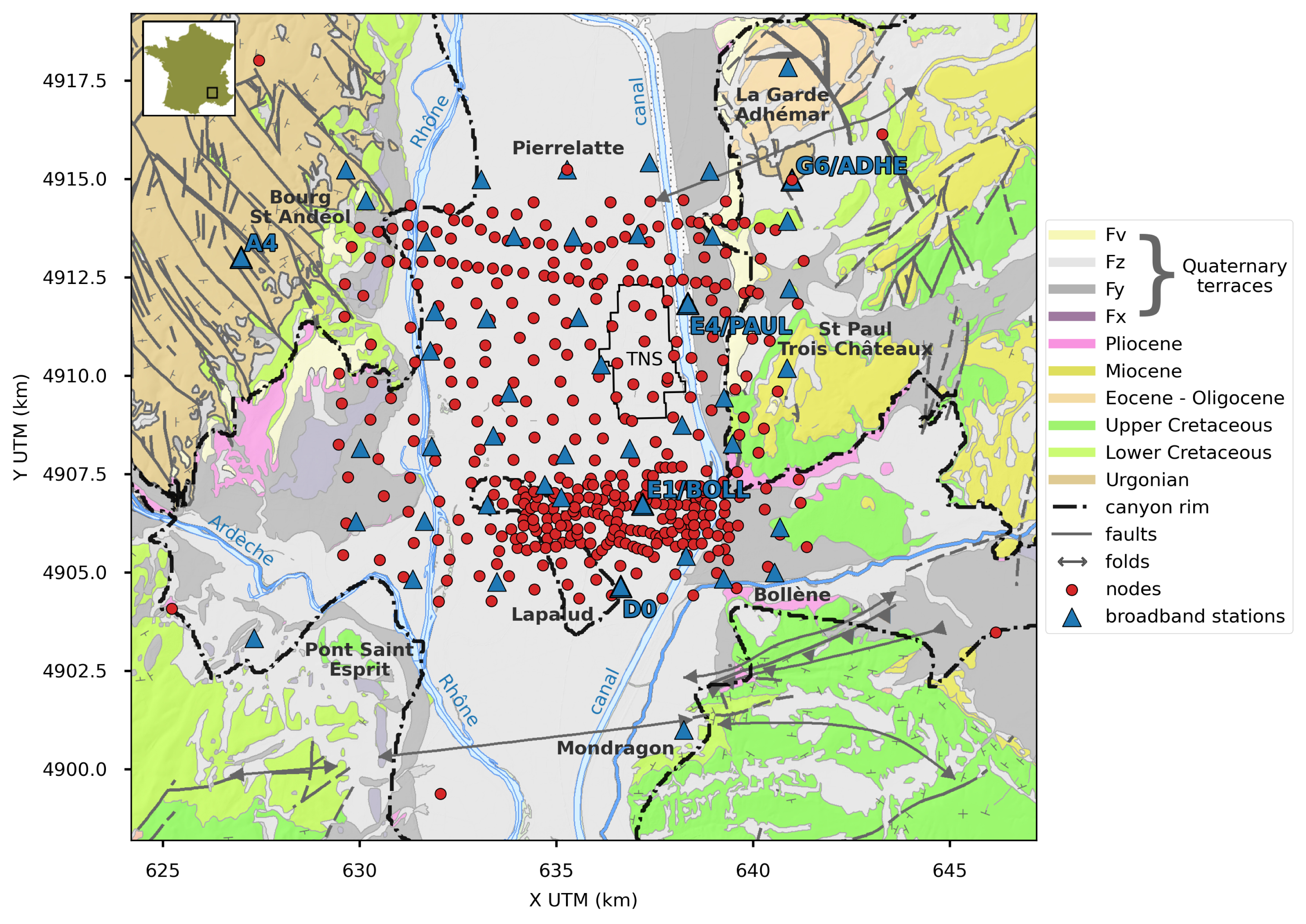
Simplified geological map of the target zone and localisation of the two deployments (red circles: nodal array, blue triangles: broadband network). Background colors correspond to main geological units (see legend). The extent of the map corresponds to the domain of interest for numerical simulations (excluding 15-km-wide margins).
From this first knowledge of the canyon, a 10 km × 10 km area surrounding the imprint of Pliocene and Quaternary sediment deposits around the TNS (Figure 1) was targeted. This extension allows us to embed the edges of nearby outcrops of Cretaceous series incised by the canyon, that constitute the basement of the canyon sedimentary in-filling. Most of this target zone is located in a heavily industrialized area, including the widespread TNS, a hydroelectric dam, towns, several railroads and a highway. The associated anthropogenic activity controls the distribution of high-frequency noise sources locally [Gisselbrecht et al., 2023].
Two complementary seismic campaigns were carried out in the framework of the DARE project [Froment et al., 2022b]. The first campaign consisted of deploying 400 3-component seismic nodes over a 10 km × 10 km area for one month (red dots in Figure 1). This campaign targeted the recording of seismic ambient noise. A second campaign consisted of deploying about 50 broadband stations over the same target area for more than eight months and targeted the recording of seismicity (including teleseismic events, regional, and local seismicity). These two datasets [Pilz et al., 2021, Froment et al., 2023b] are presented in detail in a data paper [Froment et al., 2022b] and are publicly available (see section Data and software availability).
The present study exploits the ambient noise data recorded by the 400-node network. In the methodological approach adopted in this work, seismicity data recorded by the 50-station network will only be used here to compare our numerical estimations of seismic amplification with observations. Three-component Geospace GSX nodes have been used for the dense nodal experiment whose design is shown in Figure 1. The average inter-node distance is about 800 m over the area. About half of the stations spaced 200–250 m apart are used to form a denser grid located south of the TNS. Similarly, two dense east–west lines following two roads are located north of the TNS. Information about data completeness, noise levels, and overall data quality is available in Froment et al. [2022b]. A detailed characterization of seismic noise sources recorded by the nodal network is given in Gisselbrecht et al. [2023].
3. Soil model from noise-based medium characterization
3.1. 3D VS model from ANSWT
As mentioned in the introduction, the dataset of continuous seismic noise recorded by the nodal array was processed using a standard ANSWT workflow to obtain a 3D model of shear-wave velocity, as presented in Froment et al. [2022a]. In order to bring elements for the discussion of the results obtained by using this model, we detail the workflow used in this previous work hereafter:
- Cross-correlations of seismic signals between all pairs of stations of the nodal array (except 6 nodes located outside the dense 10 × 10 km grid, and 24 nodes with unusable data, resulting in 69,192 valid cross-correlations). Continuous signals were cross-correlated over 30-min-long time windows after spectral whitening, and stacked over the one-month duration of the acquisition. The cross-correlations of all three components (N,E,Z) provided the full cross-correlation tensor. Inter-station cross-correlations were then rotated in terms of radial (RR) and transverse (TT) components assuming straight inter-station paths. The vertical components (ZZ) of the cross-correlations were used for exploiting Rayleigh waves and the transverse (TT) for exploiting Love waves.
- Semi-automatic picking of fundamental-mode group-velocity dispersion curves using frequency-time analysis [FTAN, Dziewonski et al., 1969, Levshin et al., 1989]. A statistical quality control of the picked dispersion curves was used to reject outliers falling outside two standard deviations of the distribution of picked values. After this quality control, a total of 17,031 Love dispersion curves between 0.4 and 3 Hz and 29,719 Rayleigh dispersion curves between 0.35 and 6.5 Hz were kept for tomography (i.e., 25% and 43% of the full dataset, respectively). The tomography is therefore considered to be well constrained up to 3 Hz (by both Love and Rayleigh data) and partially constrained up to 5–6 Hz (only by Rayleigh data).
- Frequency-dependent 2D traveltime tomography [Barmin et al., 2001] in order to convert inter-station dispersion curves into local dispersion curves, i.e. build group velocity maps. This step was performed via a linearized inversion involving regularization in the form of norm damping and lateral smoothing. The choice of these regularization parameters plays a role in the resolution of the final model.
- Inversion of local group-velocity dispersion curves into local 1D VS profiles using a Neighbourhood Algorithm [Sambridge, 1999, Mordret et al., 2014]. Here the use of a global optimization scheme allowed for a statistical exploration of the model space and provided an average of best-fitting models for each 1D VS profiles, which were then linearly interpolated into a 3D VS model.
The tomographic process was guided by assumptions derived from the geological knowledge at the time of this first imaging. In particular, for the 1D depth inversion (step 4), the expectation of a strong velocity contrast between sediments and bedrock led to a parameterization of the 1D profiles consisting in two smooth layers (represented by splines functions) potentially separated by a velocity discontinuity (if required by the data). This parameterization was adapted locally within sub-areas defined by clustering the local dispersion curves after the 2D tomography stage (step 3), using a data-driven K-means algorithm [MacQueen, 1967]. The resulting four sub-areas are shown in Figure 2 and turn out to well coincide with previous geological knowledge. Area #1 (in blue in Figure 2) corresponds to the deepest parts of the basin. Area #2 (in green) corresponds to the shallower northwestern edge of the basin, including the northwesternmost corner where Urgonian limestones are outcropping. Area #3 (in yellow) corresponds to the eastern edge and its outcrops of post-Urgonian/pre-Messinian formations (limestones, sands, sandstones, and marls of Aptian to Miocene ages). Finally, Area #4 corresponds to a complex zone, including the so-called Lapalud island, formed by post-Urgonian Cretaceous units (limestones, sandstones and marls of Aptian to Turonian ages) expected to have lower seismic velocities than the hard Urgonian limestones [e.g., Bagayoko, 2021, Do Couto et al., 2024]. In addition to adapting the parameterization of the 1D inversion in these sub-areas, the sub-arrays were also used to perform FK analysis and estimate an average phase velocity curve that was used to constrain the 1D depth inversion of local group velocity curves within each sub-area.
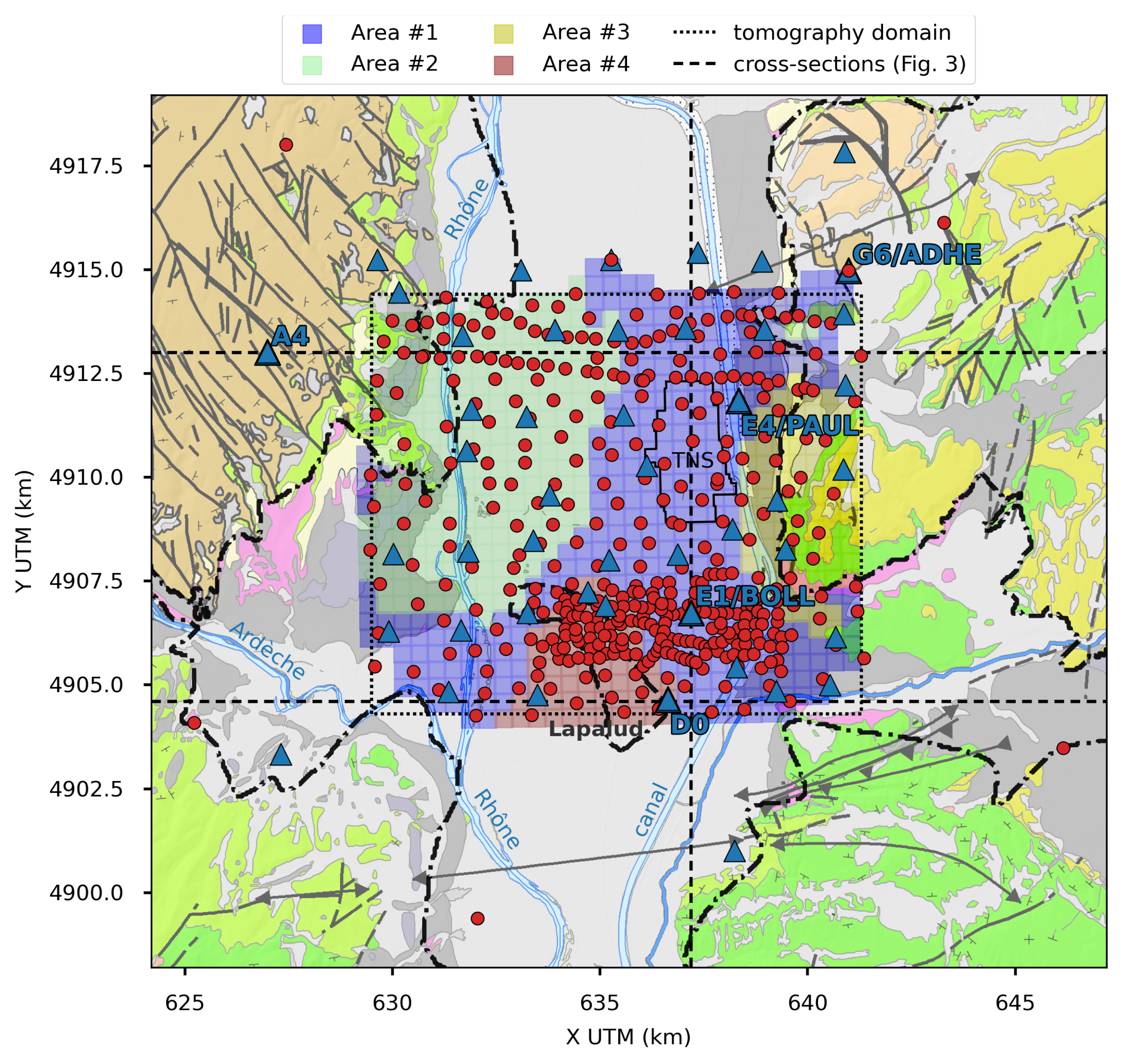
Regionalization of the tomographic domain in sub-areas based on the clustering of local dispersion curves.
Besides the assumption of a two-layer model with smooth velocity variations within each layer, we did not impose any strong constraint to the inversion. This preliminary 3D VS model is therefore mainly data driven, its purpose being precisely to investigate how such a model, based on seismic noise only via a blind ANSWT workflow, can be used to predict seismic amplification in the basin. This remains a fairly open question, considering that the ANSWT procedure uses phase information only (amplitudes are discarded by spectral whitening in the cross-correlations).
In order to use the ANSWT model for numerical simulations, the 3D VS volume is extrapolated outside the tomographic domain, both laterally and vertically, to define seismic properties in the full simulation domain, which extends laterally by 15 km from the limits of the domain of interest (SEM domain in Figure 2), and vertically down to 30 km depth. Because, in a first time, we want to rely on our data-driven ANSWT model and avoid making strong assumptions about the subsurface, lateral extrapolation is performed invariantly at a given depth. Downward vertical extrapolation consists in a smooth transition from the bottom of the tomographic model (1000 m below ground surface) to a constant velocity of 3000 m/s at 1500 m depth. This value of VS = 3000 m/s is chosen for consistency with prior measurements in the area [Gélis et al., 2022]. It also roughly corresponds to the maximum velocity of the tomographic model at 1 km depth, and therefore ensures a positive velocity gradient with respect to depth. Outside the basin, we also perform a vertically invariant extrapolation upwards in order to assign seismic properties to topographical heights above basin level.
Figure 3 gives several views of the obtained 3D VS model. Figure 3a gives a 3D view that includes N–S and E–W vertical cross-sections through the VS model (left and back panels, first colorbar), as well as the 1200-m/s iso-velocity surface that can be associated to the interface between sediments and bedrock (second colorbar). Figure 3b gives a 3D view of the numerical model, after extrapolation of the ANSWT model outside the tomographic domain over the full domain of interest (but excluding 15-km-wide margins, which just consist of further extrapolation). Figure 3c shows a vertical N–S cross-section along the expected axis of the Rhône paleo-canyon [Gélis et al., 2022, Froment et al., 2022a], passing through the TNS and through station E1/BOLL [on which we will focus later on to illustrate our results, and compare them with those of Gélis et al., 2022]. Figure 3d shows a vertical E–W cross-section in the south of the tomographic domain, through the Lapalud island and station D0 (on which we will also focus later on to illustrate our results).
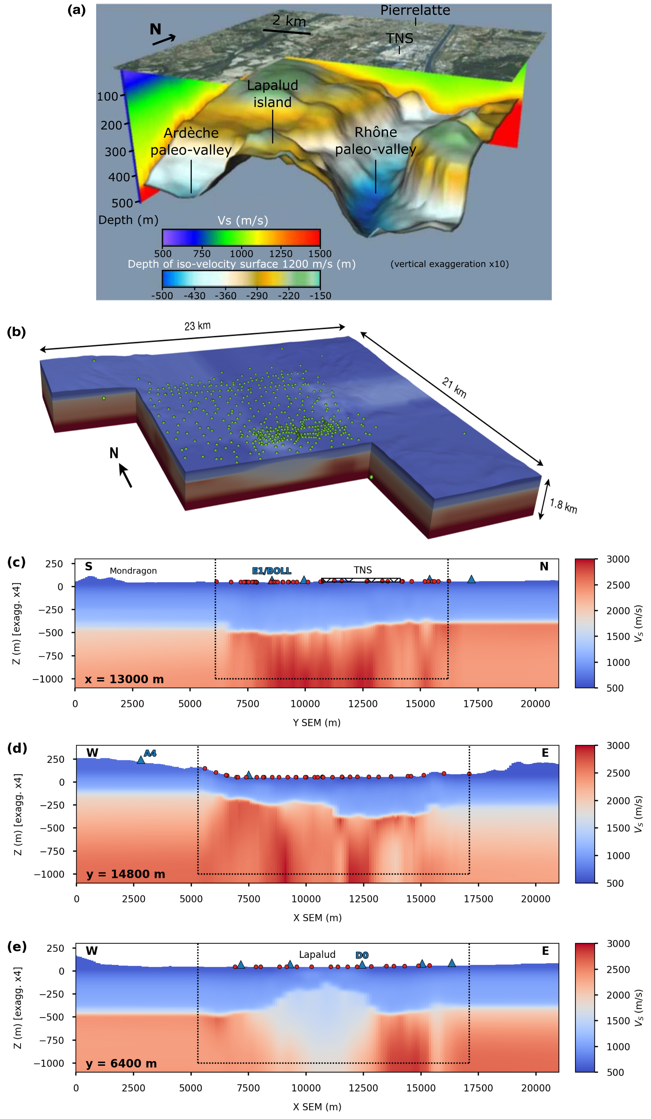
3D Vs model. (a) 3D view showing the interface between sediments and bedrock [adapted from Froment et al., 2022a]. (b) 3D view of the numerical model after extrapolation outside the tomography domain (excluding 15-km-wide margins). Green dots represent nodes and broadband stations. (c) South–north vertical cross-section along the axis of the paleo-Rhône canyon. (d) West–east vertical cross-section through the northern part of the array and station A4. (e) West–east vertical cross-section through the southern part of the array and the Lapalud island. In (c–e), the dashed box corresponds to the tomography domain. Red dots and blue triangles represent nodes and broadband stations located within 500 m of the sections (see Figure 2 for the location of the sections). Masquer
3D Vs model. (a) 3D view showing the interface between sediments and bedrock [adapted from Froment et al., 2022a]. (b) 3D view of the numerical model after extrapolation outside the tomography domain (excluding 15-km-wide margins). Green dots represent nodes and broadband stations. ... Lire la suite
As already described by Froment et al. [2022a], the ANSWT VS model agrees well with the main geological structures expected in the area. In particular, the range of estimated shear-wave velocity values are consistent with previous studies [e.g., Gélis et al., 2022], with values ranging from 500 to about 1200–1400 m/s in the sediments, and from about 1700–2000 to 3000 m/s in the underlying bedrock. Moreover, the velocity discontinuity between the two layers (which roughly corresponds to the 1200-m/s iso-velocity surface shown in Figure 3a) coincides well with the expected depth of the paleo-canyon, at least for its deeper parts, with a north–south axis corresponding to the paleo-Rhône and a southwestern branch corresponding to the paleo-Ardèche (Figure 3a). Between these two branches, the model also depicts the so-called Lapalud island with higher velocities reaching shallower depths, representing post-Urgonian Cretaceous units (Figures 3a,c).
However, when looking in more detail, we notice that some features of the model are questionable. In particular, the model does not display high velocities reaching the surface, even in regions where we expect surface outcrops of Cretaceous formations (especially in the northwestern corner and on the eastern edge of the basin, Figures 3a,b). Instead, the model exhibits a lower-velocity layer (500 < Vs < 1000 m/s) with a thickness of at least 200 m over the entire domain (Figures 3b–d). This low-velocity layer is not restricted to the basin, which is therefore not well delimited laterally. We will see in the following that this lack of basin edges will have consequences in terms of seismic amplification.
In spite of these limitations, the fact that the 3D VS model derived from ANSWT well depicts the expected large-scale geometry of the Messinian paleo-valley at depth, including some complex structures such as the Lapalud island, motivates us to use this model for numerical simulations, in order to look at the seismic amplification that it may generate. This, however, first requires the definition of other seismic properties in the considered 3D volume. We will now present how we define these properties, and we will distinguish between properties that are constrained by the same seismic noise data as the VS model (namely QS) and other properties that are estimated by other means (VP, density, QP).
3.2. Estimation of shear-wave quality factors QS
Besides ANSWT, the seismic noise recorded by the dense array is processed via Q-SPAC analysis [Prieto et al., 2009] to estimate seismic attenuation parameters (QS), following the methodology of Boxberger et al. [2017]. To this end, the study area is subdivided into 15 sub-arrays, each of them containing 15 to 25 seismic nodes.
In a first step, the Extended Spatial AutoCorrelation (ESAC) method is adapted to first obtain mean 1D VS profiles below each sub-array by joint inversion of Rayleigh wave dispersion and H/V spectral ratios, and then estimate frequency-dependent Rayleigh-wave attenuation factors from the mean 1D VS profiles [Ohori et al., 2002, Boxberger et al., 2011]. In a second step, individual 1D QS profiles are obtained from the inversion of the Rayleigh-wave attenuation coefficients by constraining the VS profiles to the values obtained in the first step, following Xia [2014]. It is worth noting that the seismic attenuation discussed here does not distinguish between intrinsic and scattering attenuation. Furthermore, while the Rayleigh-wave attenuation factors of the input data depend on frequency, the QS parameter of the obtained layered model is assumed to be frequency-independent. Finally, following Xia et al. [2002], we disregard the contributions of P waves on the Rayleigh-wave attenuation factors.
In the end, 15 layered 1D profiles representative of average VS and QS values as a function of depth are derived, one for each of the 15 sub-arrays of the nodal network. VS profiles are found to be in general agreement with the ANSWT model (with deviations smaller than 15%). These profiles are used to calibrate a relationship between VS and QS values in the form of a 6-order polynom [after Taborda and Bielak, 2013, see Figure 4] which is then used to derive a 3D QS model from the 3D ANSWT VS model. This is expected to provide more realistic and site-specific QS values than assuming generic relationships (e.g., VS/QS = 10), or other relationships from the literature calibrated for other sites [e.g., Taborda and Bielak, 2013, see Figure 4]. The QS values obtained from our site-specific relationship range from 21 for small VS values in shallow sediments to 360 for high VS values in the deep substratum (Table 1).
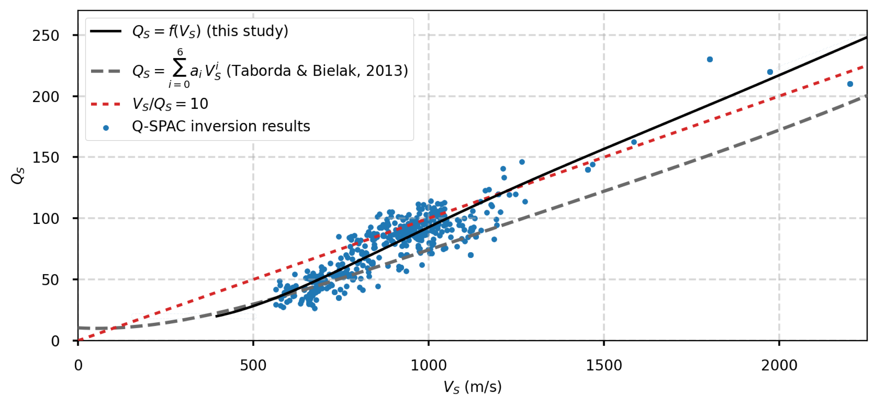
Calibration of a site-specific VS/QS relationship using Q-SPAC inversion results.
Ranges of seismic properties in the two layers of the 3D VS model
| VS (m/s) | VP (m/s) | Density (kg/m3) | QS | QP | ||||||
|---|---|---|---|---|---|---|---|---|---|---|
| min | max | min | max | min | max | min | max | min | max | |
| 1st layer (sediments) | 500 | 1400 | 2000 | 2675 | 2075 | 2225 | 21 | 130 | 260 | 350 |
| 2nd layer (bedrock) | 1700 | 3070 | 3075 | 5300 | 2300 | 2640 | 170 | 340 | 420 | 760 |
3.3. Other seismic parameters (VP, QP, density)
Unlike VS and QS properties, P-wave velocity VP and quality factor QP, and density parameters are not (or poorly) constrained by our ambient noise data, which are typically dominated by surface waves.
In situ geotechnical measurements performed in the vicinity of the TNS down to approximately 30 m depth provide us with local estimations of VP, VS, and density [Moiriat, 2019]. These measurements show VP/VS ratios of up to 8 in very shallow sediments (Quaternary limons and alluvions forming thin (<20 m) layers and lenses, which are not included in the ANSWT due to its lack of sensitivity to these shallow layers), and of about 4 for values of VS ≈ 500 m/s in the blue marls encountered below 15 to 20 m depth. It is worth noting that these values of VS ≈ 500 m/s are in very good agreement with the VS values of the shallow part of the basin in the ANSWT model which, according to the smallest wavelength considered in the tomography (≈100 m), we can regard as effective VS values for the basin sediments in the first 30 to 50 m.
Based on these geotechnical measurements, we calibrate a site-specific VP/VS relationship of the form
| (1) |
In lack of sufficient density measurements, we use Gardner’s empirical law [Gardner et al., 1974, equation (7); Brocher, 2005, equation (2)] in order to relate density to P-wave velocity VP. This law is supposed to be valid for sedimentary rocks such as limestones. We verify that the density values obtained for the range of seismic velocities encountered in our ANSWT model roughly coincide with expected values for the known lithologies in the area (limestones, sandstones, and marls), as well as with the abovementioned geotechnical measurements.
Finally, we must define values for the P-wave quality factor QP in our 3D model, although this parameter is expected to have very little impact on the amplification of the SH excitation that we will simulate. In lack of any constraint on these QP values, we derive them from QS, VS, and VP values, under the assumption that the compressibility quality factor is much larger than the shear quality factor [Q𝜅 ≫ Q𝜇, Dahlen and Tromp, 1998, equation (9.59), p. 350].
Table 1 summarizes the ranges of values of the different seismic properties in the final 3D seismic model.
4. Numerical estimation of seismic amplification
4.1. Simulation of seismic wave propagation
Simulations of seismic wave propagation in the constructed 3D model are performed using the EFISPEC software [De Martin, 2011], which makes use of a time-domain spectral-element method (SEM) solving the 3D equation of motion in visco-elastic media. A hexahedral mesh is designed for simulations valid up to 5 Hz, which is about the maximum frequency used to constrain the ANSWT model (at least with Rayleigh data, see Section 3.1). The simulation domain extends laterally 15 km further than our domain of interest (Figures 1 and 2) and vertically down to 30 km, in order to mitigate parasite reflections on domain boundaries, where the absorbing condition is based on a paraxial approximation [Stacey, 1988]. This leads to a total of 6.5 M elements, with an element size that varies between 100 m and 300 m from the shallow to the deeper parts of the model. In order to reproduce the assumptions underlying SSR calculations, the simulated source is a vertically-incident plane wave with SH polarization in the X- (east–west) or Y - (north–south) direction, injected at 5 km depth. We perform two simulations, one for each polarization of the plane wave, for a duration of 60 s. Each simulation costs 3500 CPUh and is parallelized on 480 cores. The source time function is a low-pass-filtered Dirac delta function, filtered below 5 Hz, such as to remain in the domain of validity of the simulation (and of the ANSWT model) and to be able to visualize and exploit simulated outputs directly, without filtering them at the post-processing stage.
Figure 5 shows snapshots of the simulated wavefield on the free surface at different times. The vertically-incident plane wave first arrives after approximately 2.2 s of simulation in the northwestern corner, which has slightly higher velocities than the rest of the domain (Figure 5a). At 2.5 s, amplitudes are saturated over the entire domain while the plane wave is reflecting on the free surface (Figure 5b). At 3.5 and 4 s (Figures 5c, d), high amplitudes are visible in the deepest parts of the basin, reflecting 1D basin amplification due to vertical body-wave resonance, but also outside the tomographic domain, due to topographic effects, in particular on the margins that are not constrained by the tomography. After 4.5 s (Figures 5e, f), late reverberations are slightly visible in the basin (likely due to reflections on the edges of the basin), but also in the margins of the model outside the tomographic domain (due to topographic effects). These snapshots show that waves are not efficiently trapped in the basin, as we would expect in a well-delimited basin [e.g., Chaljub et al., 2015, De Martin et al., 2021]. Instead, waves escape in the low-velocity shallow layer, resulting in an amplification over the entire domain, in particular in the margins of the simulation domain that are not constrained by the tomography.
Snapshots of the simulated wavefield (vy component excited by a vertically-incident SH plane wave polarized in the Y direction) on the free surface at different times. The black contour corresponds to the iso-depth 375 m of the velocity discontinuity between sediments and bedrock, delineating the deepest part of the basin. The dashed line corresponds to the tomographic domain. The full movie of wave propagation is provided in Supplementary Material.
Based on these first observations and despite some limitations, we will now continue to analyse our simulation results, especially in terms of predicted amplification, with the objective to better understand the limitations of our ANSWT model, which we just started to point out, and thus to draw perspectives about how such ANSWT models could be improved to better reproduce basin amplification. We propose to start by looking into the seismograms simulated at the locations of known stations, including E1/BOLL that has been investigated by Gélis et al. [2022], as well as A4 that serves as a reference station for the calculation of our empirical, earthquake-based SSR (see Supplementary Material for more details). We shall specify here that station A4 is located on the same kind of Urgonian outcrop and presents similar H/V characteristics as station G6/ADHE that was used as a reference station by Gélis et al. [2022].
Figure 6 shows seismograms (Figure 6a) simulated at stations E1/BOLL (in blue) and A4 (in orange) and their amplitude spectra (Figure 6b). In Figure 6b, thin lines represent raw spectra and thick lines represent spectra smoothed using Konno-Omachi smoothing with a bandwidth b = 40 [Konno and Ohmachi, 1998] which are then used to compute spectral ratios (Figure 6c). As expected, the signal simulated at station E1/BOLL has a long duration because of wave reverberations in the basin (only the first 11 s of the signals are shown in Figure 6, but reverberations generate non-negligible amplitudes—of the order of about 10% of the maximum peak amplitude—over the entire 60-s duration of the simulation). The signal simulated at station A4, on the other hand, does not correspond to our expectations for a reference rock site precisely because it also contains late reverberations of similar, non-negligible amplitudes as station E1. Apart from a high-amplitude arrival at about 4 s, probably due to a vertical body-wave reflection in the basin, the ground motion in E1 does not seem much amplified compared to the one in A4. In the Fourier domain (Figure 6b), the amplitude spectra at stations E1 and A4 differ mostly by the frequencies of their respective peaks at low frequencies: around 0.5 Hz for E1 (blue line in Figure 6b), which corresponds well to the 1D resonance of the basin [Gélis et al., 2022], and around 1 Hz for A4 (orange line in Figure 6b), which rather corresponds to the 1D resonance of the shallow low-velocity layer extrapolated outside the actual extent of the basin (if we consider a relation between resonance frequency fres and layer thickness h of the form
(a) Seismograms simulated at stations E1/BOLL (in blue) and A4 (in orange) and their amplitude spectra (b), for a vertically-incident plane wave source polarized in the Y direction (vy components are shown). Green curves show the reference signal considered for computing amplification, which corresponds to the recording of the incident plane wave at 10 km depth. (c) Spectral ratios.
As a consequence, we cannot consider the signal simulated at A4 as a reference for estimating amplification via spectral ratios: the resulting amplification would be dramatically underestimated, especially at frequencies corresponding to the 1D resonance of the shallow low-velocity layer (e.g., 1 Hz, see red curve in Figure 6c). Instead, we consider a deep reference point, located at 10.050 km depth, i.e., at the same distance from the depth at which the plane wave source is injected (5 km) as the free surface in the basin (which has an average elevation of 50 m asl). The seismogram extracted from this deep reference point is time-windowed, such as to retain only the incident plane wave, which has travelled in a homogeneous medium between its injection point at 5 km depth and this reference point at 10.050 km depth, therefore yielding a clean signal (green curves in Figure 6). The amplitude spectrum of this windowed signal is then multiplied by 2, which corresponds to the amplitude spectrum of a point that would be located on the free surface. In doing so, we therefore define a reference amplitude spectrum that is equivalent to the theoretical response of a point on the free surface above a homogeneous halfspace that would have the same seismic properties as the deep part of our 3D numerical model (including visco-elastic attenuation, which makes this deep reference spectrum different from the spectrum of the injected source time function) and that is consistent with the wavefield simulated at the free surface (since it is extracted from the simulated wavefields, and not computed separately). We refer to the spectral ratio computed with this deep reference as the amplification function (AF), as opposed to the standard spectral ratio (SSR) computed with a reference point located on the free surface. We have verified that AF and SSR are identical in the case of a surface reference point located above a homogeneous subsurface, and far away from basin edges (clean numerical reference). As a consequence, our numerical amplification functions remain comparable to empirical SSRs computed with respect to a clean empirical reference on the field, which is the case of station A4. Figure 6c shows the resulting amplification functions for station E1 (in blue), with a clear peak around 0.55 Hz corresponding to basin resonance, and for station A4 (in orange), with a peak at 1 Hz, related to the resonance of the artificially extrapolated low-velocity layer. In the following, we will now analyse in more detail these numerical amplification functions, with a particular focus on points located in the basin (since we know that rock sites outside the basin are misrepresented in our model, and therefore may provide less relevant amplification results).
4.2. Numerical amplification
In this section, we will analyse in three different ways the numerical amplification simulated in our ANSWT model. First, we will compare our numerical amplification functions and their spectral characteristics to empirical SSR measurements based on earthquake data recorded during the deployment of the DARE broadband network. We will exemplify this comparison at two specific locations in the basin, which we have identified as representative of two different signatures that we find of particular interest for our scope, especially when compared to a 1D SH response approximation, which we will also provide as another point of comparison. Second, we will comment on the spatial variability of the numerical amplification predicted in our model, for a few example frequencies. Third, we will have a closer look at this spatial variability at low frequency, and more precisely at the spatial pattern of the (mis)match between our numerical amplification and two empirical amplification estimations based on earthquake and noise data.
4.2.1. Local comparison of numerical amplification with earthquake-based SSR and 1D amplification
Figure 7 shows the amplification at stations E1 (a) and D0 (b) as a function of frequency (see Figure 1 for the location of these two stations). Purple lines represent the empirical, earthquake-based SSR computed with respect to reference station A4 and their uncertainties (purple dashed lines). A catalog of these empirical SSR for all stations of the DARE broadband network is provided in Supplementary Material, together with details on the computation of these SSR. The green line corresponds to the SH amplification computed in a 1D model extracted from the 3D model below the station of interest (right panels), using the gpsh function of the Geopsy software [Wathelet et al., 2020]. The numerical amplification of the horizontal component (AFH) computed in the 3D tomographic model is shown as dark blue and red dashed lines for vertically-incident plane wave sources polarized in the E–W (PWX) and N–S (PWY) directions, respectively. The set of grey curves corresponds to the amplification of the horizontal component for plane wave sources polarized in different directions (PW𝜃, with 𝜃 the polarization azimuth), showing the variability of the amplification with respect to source polarization. These curves are obtained by a linear combination of the two wavefields simulated for plane wave sources polarized in the X and Y directions, in order to reproduce, by linearity of the wave equation with respect to the source, the wavefield generated by a plane wave source polarized in any given direction.
Amplification spectra at stations E1 (a) and D0 (b). Dark blue and red dashed lines: numerical amplification of the horizontal component (AFH) in the 3D tomographic model, for vertically-incident plane wave sources polarized in the E–W (PWX) and N–S (PWY) directions, respectively. Grey curves: amplification of the horizontal component for plane wave sources polarized in different directions (PW𝜃). Green line: 1D SH amplification
Amplification spectra at stations E1 (a) and D0 (b). Dark blue and red dashed lines: numerical amplification of the horizontal component (AFH) in the 3D tomographic model, for vertically-incident plane wave sources polarized in the E–W (PWX) and ... Lire la suite
The two stations considered in Figure 7, E1 and D0, exhibit two different amplification patterns that can be linked to their respective locations in the basin, and eventually to the corresponding subsurface structures. Below station E1, we know from previous studies that the paleo-canyon is quite deep [about 560 m according to Gélis et al., 2022], and that a thick pile of Pliocene sediments probably lies directly on top of the hard substratum of Urgonian limestones. This results in a significant observed amplification (up to 7 ± 2) above the main resonance frequency of the canyon (about 0.5 Hz for this location/depth, according to Gélis et al. [2022]. Here it is worth noting that the numerical results do not retrieve this observed level of amplification (with a maximum of about 4 ± 1), nor its broadband character: while the observed amplification exhibits a plateau above 0.55 Hz, which is commonly interpreted as the signature of 3D wave propagation effects [due, in particular, to laterally propagating surface waves generated at the edges of the basin, see e.g. Cornou and Bard, 2003, Bindi et al., 2009], the numerical amplification computed from 3D numerical simulations (envelope of gray curves) remains quite close from the 1D resonance peaks predicted in a local 1D model extracted below the considered station (green curve). This suggests that the ANSWT model does not generate significant amounts of laterally propagating surface waves within the basin, which can be easily understood from our observations of the model (Figure 3) and of the wavefield (Figure 4), where we already noted the lack of clear lateral basin edges, resulting in a lack of wave trapping within the basin. Nevertheless, the numerical amplification computed in the 3D ANSWT model is not strictly identical to a 1D amplification. In particular, it exhibits non-negligible variations with respect to source polarization for some frequencies, including in the vicinity of the main resonance frequency (0.45–0.55 Hz). While this source-related variability would probably deserve a more detailed investigation [e.g., Maufroy et al., 2017], it is a clear indication that the ANSWT model well includes some 3D characteristics of the basin that cannot be captured by purely 1D approximations. Moreover, it should also be noted that the local 1D profile extracted from the 3D ANSWT model below station E1 and the associated 1D amplification (green curves in Figure 7a) are very similar to the results obtained by Gélis et al. [2022, their figure 8d] for this location. This suggests that the ANSWT well played its role in terms of local VS estimation, just as well as the local Ambient Vibration Analysis performed by Gélis et al. [2022], but with the added value of imaging the lateral variations of the 1D VS structure in the basin.
Regarding station D0, it is located at the border of the Lapalud island, where the subsurface has a complex structure due to the presence of the late lower Cretaceous units in between the Pliocene sediments and the Urgonian bedrock [Bagayoko, 2021, Do Couto et al., 2024]. These units are made of sandstones and marls, and have intermediary seismic velocities compared to the Pliocene and Urgonian lithologies, which in the VS profiles is represented by a smooth gradient of velocity progressively increasing with depth. This results in a lower level of observed amplification (up to 3 ± 0.5). This amplification also displays a broadband character as a function of frequency, but for a different reason as previously: in this case, the amplification plateau above 0.5 Hz is due to the smooth gradient of increasing velocity with depth, and not to 3D wave propagation effects (since 1D amplification also shows this broadband character). Interestingly, both 3D and 1D numerical results show a good agreement with the observations in this case, which again suggests that the amplification is not dominated by 3D propagation effects at this location, but by 1D vertical resonance, so that the 1D approximation is sufficient to explain the observations. It should be noted, however, that this agreement is only possible because the tomography well played its role in terms of (3D) characterization of the local (1D) velocity structure.
4.2.2. Spatial variability of the numerical amplification
One of the interests of numerical simulations is to provide access to the spatial variability of the amplification in the basin. Figure 8 shows amplification maps at different frequencies. At 0.5 Hz, most of the amplification corresponds to the deepest part of the basin (delineated by the iso-375-m depth contour of the interface between sediments and bedrock), as expected. At higher frequencies, however, amplification does not behave as expected. At 1 Hz, amplification is larger outside the basin than inside, which is likely due to the resonance of the shallow 200-m-thick low-velocity layer at this frequency. At 2 Hz, the amplification pattern is less clear but seems to concern mainly the slopes of the basin. At 4 Hz, results simply do not seem to be relevant, and are probably dominated by the topographic effects identified in the wavefield snapshots (Figure 5). In the following, we focus our analysis to the low-frequency part of the amplification, in the frequency range 0.3–0.7 Hz, related to the deepest parts of the basin (note however that this frequency range is wide enough to cover a relatively wide range of canyon depths, from about 300 m to 700 m). More specifically, we propose to look at the ratio between our numerical amplification and the observed amplification in this frequency range, for all broadband stations (earthquake-based SSREQ, Figure 9) and all nodes (noise-based SSRn, Figure 10).
Maps of the amplification of the horizontal component at 0.5, 1, 2, and 4 Hz, for a vertically-incident SH plane wave polarized in the Y direction (N–S). The black line represents the iso-375-m depth contour of the interface between the two layers considered in the 1D depth inversion. Margins outside the tomographic domain have been masked.
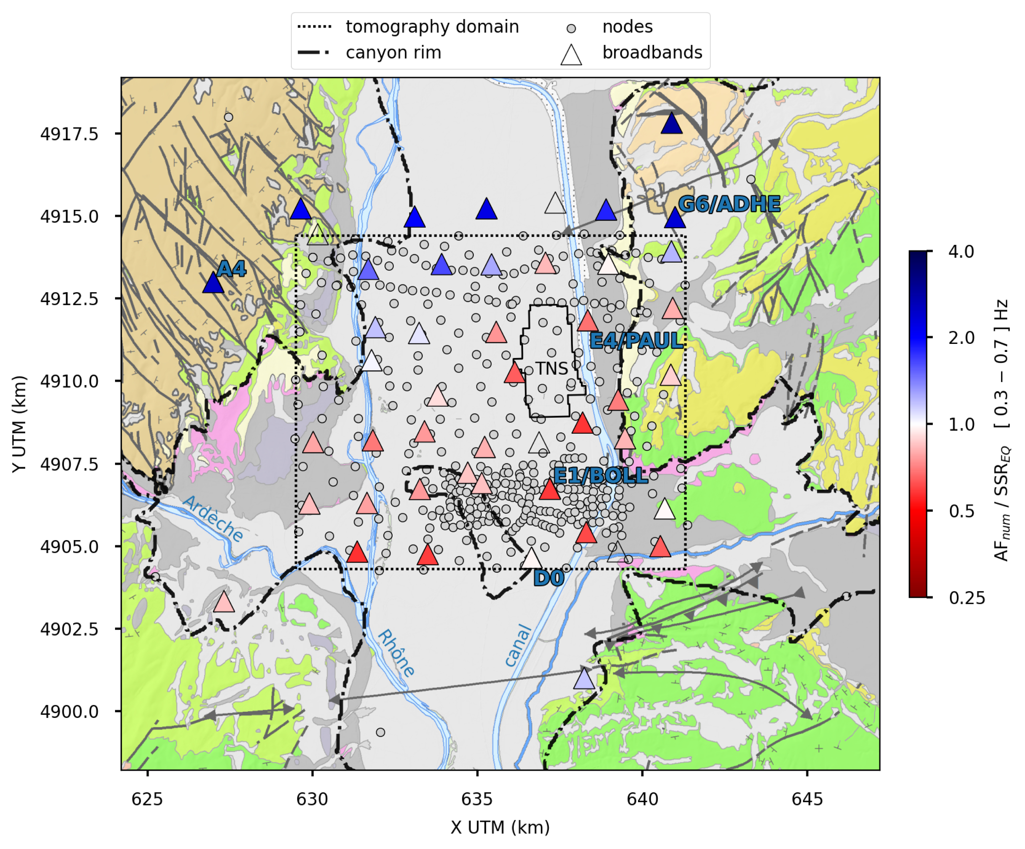
Mean ratio between numerical amplification and earthquake-based SSREQ between 0.3 and 0.7 Hz (note the logarithmic color scale).
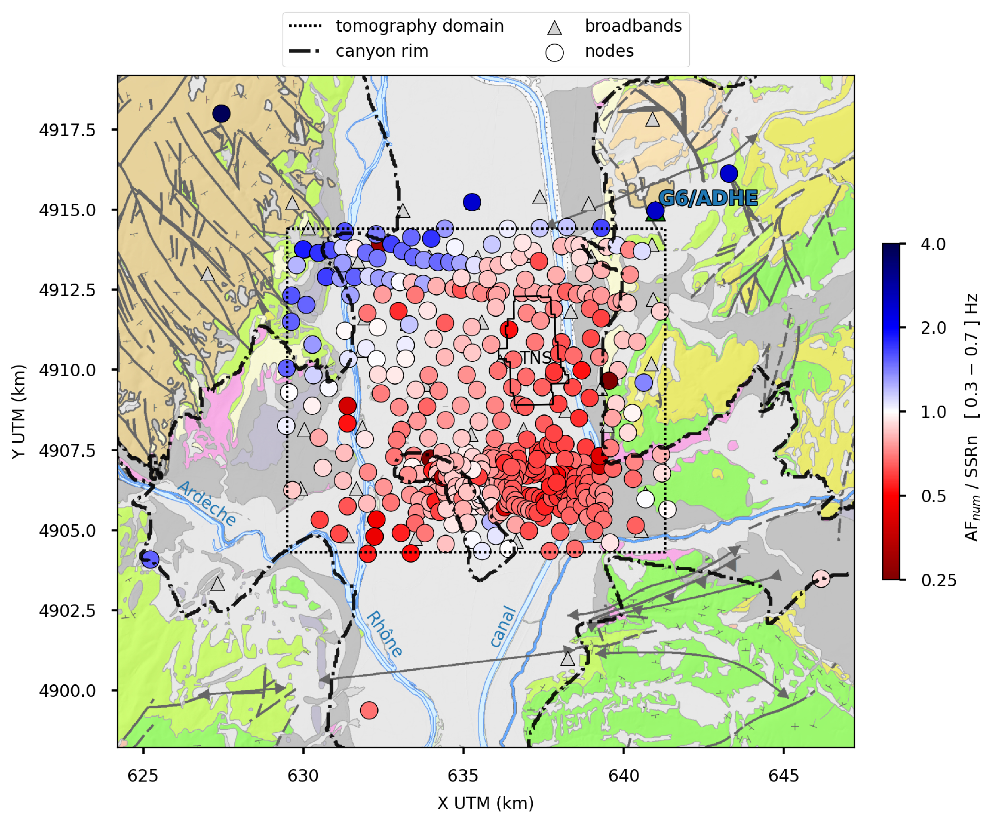
Mean ratio between numerical amplification and noise-based SSRn [Gisselbrecht et al., 2023] between 0.3 and 0.7 Hz (note the logarithmic color scale).
4.2.3. Spatial variability of the misfit between numerical amplification and observed SSR
Comparison to earthquake-based SSREQ
Figure 9 shows the spatial distribution, for all broadband stations, of the mean ratio between our numerical amplification AFnum (log-average of the gray curves in Figure 7) and the observed earthquake-based amplification SSREQ with respect to reference station A4 in the frequency range 0.3–0.7 Hz. According to the logarithmic color scale, dark red and dark blue colors represent stations where the numerical amplification underestimate and overestimate the observations by a factor of 4, respectively. Empty triangles correspond to stations for which we could not estimate empirical SSREQ, due to an insufficient signal-to-noise ratio of the earthquake recordings or to a lack of data (see Supplementary Material for details). The dashed-dotted line represents the surface imprint of the canyon rim, as interpreted from geological mapping (Figure 1), which provides a visual guide to locate the results with respect to the basin. The dotted line delimits the domain constrained by the tomography, outside which laterally-invariant extrapolation is performed (Figure 3) and makes the results hardly interpretable, in particular at rock sites (e.g., A4, G6/ADHE). Within the tomography domain, however, the ratio between numerical and observed amplification is always comprised between 0.5 and 2, and is close to 1 for some stations. This suggests that the ANSWT model, although not perfect and still improvable, is able to explain, in some extent, the amplification observed in this low-frequency range, and in various parts of the basin (where, incidentally, the frequency range 0.3–0.7 Hz may include different amplification phenomena depending on the location in the basin and on the underlying/surrounding geological structures). In order to look in more detail at the spatial pattern of the (mis)match between numerical and observed amplification, we now propose to look at the ratio between numerical and noise-based amplification.
Comparison to noise-based SSRn
Similarly to Figure 9, Figure 10 shows the spatial distribution, for all nodes, of the mean ratio between our numerical amplification AFnum and the observed noised-based amplification SSRn in the frequency range 0.3–0.7 Hz, in which we consider SSRn estimations to be reliable [Gisselbrecht et al., 2023]. Indeed, several studies have reported a good agreement between noise-based SSRn and earthquake-based SSR in this frequency band [e.g., Lermo and Chávez-García, 1994, Bard, 1999], mostly because distant sources dominate the ambient noise wavefield at these frequencies [e.g., Bonnefoy-Claudet et al., 2006]. In order to further mitigate undesired effects of local and transient low-frequency sources (such as wind), Gisselbrecht et al. [2023] computed these SSRn using short time windows (1 min) restricted to quieter nighttime recordings. Note also that these empirical SSRn have been estimated with respect to a node co-located with reference station G6/ADHE. The similarities between Figures 9 and 10 in the vicinity of broadband stations suggests that the two empirical estimations, based on earthquake and ambient noise, are overall consistent, and that the choice of the reference station, A4 or G6/ADHE, has very little effect on the results in this low-frequency band, as also suggested by the SSR ≅ 1 between the two stations (see Supplementary Material). Thanks to the density of the nodal array, Figure 10 gives a nice spatial view of the (mis)match between empirical and numerical amplification, and enables to look at its spatial pattern in more detail.
In particular, we see again that our numerical amplification over-estimates the observations in the northwesternmost corner of the domain, including at rock sites where we know that Urgonian limestones are outcropping, but also in the north-west of the basin (south-west of Pierrelatte), suggesting that the ANSWT model might over-estimate sediment thickness in this area. In contrast, amplification seems under-estimated in the deepest part of the basin, along the north–south axis of the paleo-Rhône canyon, as well as along the paleo-Ardèche in the south-west of the domain. Knowing that ANSWT provides a similar estimate of the canyon depth at station E1 as AVA [Gélis et al., 2022], this underestimation could suggest a lack of 3D wave propagation effects in these parts of the model, all the more that they also correspond to regions susceptible to be affected by laterally propagating surface waves generated at basin edges.
Interestingly, one of the areas where the match between numerical and empirical amplification seems the most satisfying corresponds to the Lapalud island in the South of the domain. Again, this suggests that the ANSWT model is successful in estimating the subsurface velocity structure in this region, despite its relative complexity due to the presence of heterogeneous post-Urgonian Cretaceous units. It also suggests that local 1D effects may be dominant in the amplification at this location, which may be intuitively understood as the fact that the top of the island itself is not affected by waves that are diffracted by (/away from) the island. The ratio between numerical and noise-based amplification is also quite satisfying north-west from Lapalud, where the basin is shallower [Do Couto et al., 2024], as well as on its eastern margin, which suggests that the post-Urgonian Cretaceous and Tertiary units that form this margin do not have the same properties as the rock sites located on Urgonian outcrops (A4, G6/ADHE), and experience some amplification compared to these hard rock sites. These lateral variations of bedrock properties, rarely taken into account in numerical studies, are important to consider, as they affect not only the local response, and thus the choice of a reference for SSR calculation [Steidl et al., 1996], but also the impedance contrast at the sediment/bedrock interface.
5. Discussion
The aim of this paper was to investigate if and how a standard ANSWT model could be used for the numerical estimation of seismic amplification in sedimentary basins. In light of our results, we can state that ANSWT is surely a method of choice for depicting the large-scale velocity structure of the subsurface, but that a standard, purely data-driven, ANSWT workflow alone is visibly not sufficient to generate seismic models that well reproduce the observed amplification in complex sedimentary basins where 3D wave propagation effects are significant.
In particular, we clearly saw the consequences of the lack of well-marked lateral basin edges, and thus of laterally propagating surface waves in the basin. There are several reasons for this lack of shallow lateral contrasts in the model, in relation to the sensitivity and resolution capacity of the surface wave data used for tomography. First, the upper layers of the subsurface (first 50 m in the basin, where the minimum wavelength is about 100 m; first 200 m outside the basin, where the minimum wavelength is about 400 m) are poorly constrained by our measurements of the dispersion of fundamental Love and Rayleigh modes in the considered frequency range (0.3–5 Hz). Second, due to this weak data sensitivity and to the relative weight of regularization (smoothing), there is a smearing of low-velocity anomalies from the center to the edges of the basin at the 2D tomography stage, all the more that the edges of the model are less well constrained by data coverage, given the imprint of the array. This understanding is important because it gives precise clues about how to improve future ANSWT applications for site effect assessment in sedimentary basins. In terms of acquisition design, it suggests that the seismic array should probably extend more outside the basin, in order to better constrain basin edges and surrounding bedrock properties. More generally, it suggests that we should seek more information about basin edges, either in the seismic data themselves or elsewhere.
In this preliminary study, indeed, we deliberately adopted a purely data-driven ANSWT approach, in order to assess its potential and limitations. But if surface wave data alone are not sufficient to generate sharp lateral variations, then we should turn to other sources of information which we first need to collect and then to integrate in the tomographic process in order to constrain our models. In our case, the surface imprint of the Messinian paleo-canyon is known from geological mapping (Figure 1), field campaigns, and borehole data. Besides, active seismic profiles are also available in the area. The interpretation of these profiles (time-domain migrated sections), together with geological field campaigns and borehole data, allows for a high-resolution identification of geological horizons [Bagayoko, 2021, Do Couto et al., 2024]. These horizons, however, cannot be considered as a strict ground truth, because the inference of their depth depends on P-wave velocity values assumed for time-to-depth conversion. Moreover, these geological horizons do not necessarily correspond to seismic impedance contrasts, as discussed in Froment et al. [2022a], and need to be interpolated over the entire domain of interest. Nevertheless, these horizons could be used as prior information in order to constrain the geometry of subsurface layers in the tomographic process. This will be the subject of further work following directly from this study, which enables us to pinpoint more precisely where this prior information should be introduced: namely both at the 2D tomography stage, where lateral coherency could be enforced using these geological constraints rather than blind smoothing, and at the 1D inversion stage, where interface depths could be constrained directly.
Finally, the computation of H/V ratios from the ambient noise data recorded by the dense nodal array also results in the estimation of an interface related to an impedance contrast that controls seismic amplification, and this information could also be worth taken into account in the tomography and in our simulations. In practice, however, how to take this interface into account is not completely obvious, given that (i) the interpretation of this interface in terms of depth also implies some assumption about VS values in the sediments, (ii) this interface may not correspond to geological stratigraphic horizons, or not always to the same horizons, and may even not be continuous [Froment et al., 2022a].
In all these cases, the consideration of such prior information in the tomographic process would be best handled in the frame of probabilistic methods, such as trans-dimensional tomography [e.g., Bodin et al., 2012, Galetti et al., 2017] or Bayesian approaches [e.g., Lu et al., 2020, Nouibat et al., 2022]. This would at least require the use of state-of-the-art imaging techniques, and probably some dedicated methodological developments as well, in particular to properly evaluate and propagate uncertainties throughout the whole ANSWT workflow, starting from reliable prior data uncertainty related to dispersion curve picking, and ending with robust posterior uncertainties on model parameters, which could then be used in our numerical simulations to explore the variability of the predicted amplification within the range of model uncertainties. As a direct perspective of this work, we are currently investigating such probabilistic methods in order to improve our tomographic model of the Tricastin basin, and explore the sensitivity of our numerical amplification to input data and model features, within realistic uncertainty ranges. Another important—and yet open—question related to data and model uncertainties concerns the frequency range in which we can reliably predict seismic amplification, based on a certain set of informations to design our numerical models.
Finally, the lack of 3D characteristics in the ANSWT model likely comes in part from the 1D approximation which the standard 2-step ANSWT procedure relies on for interpreting surface-wave dispersion in terms of velocity structure as a function of depth. This assumption could be overcome by using other imaging techniques, such as 1-step 3D ANSWT [e.g., Zhang et al., 2018] or full waveform inversion [FWI, e.g., Virieux and Operto, 2009, Lu et al., 2020]. FWI, in particular, would enable one to fully consider 3D wave propagation, as well as higher-mode surface waves, and eventually body waves (if present in the cross-correlations), that would bring additional information on the impedance contrast between sediments and bedrock, and potentially provide higher-resolution models with sharper lateral variations associated to basin edges. We would recommend the investigation of such waveform tomography techniques for building seismic models for site effect assessment as a long-term research track, keeping in mind that FWI applications in complex subsurface settings are always challenging, and that noise-based FWI is still the subject of current developments and raises challenges of its own, in particular regarding the effect of noise sources on parameter estimation [e.g., Tromp et al., 2010, Säger et al., 2018]. Standard ANSWT models such as the one considered in this study could be used as initial models for further waveform inversion approaches.
6. Conclusion
In this paper, we have used a 3D VS model of a complex sedimentary basin built via a standard ANSWT workflow to perform numerical simulations of seismic wave propagation, and compute ground motion amplification within the basin. The tomographic model well depicts the main geological structures of the basin via its lateral variations of seismic velocities at depth, but it also suffers from limitations related to surface wave sensitivity and resolution capabilities, especially in its shallow part. In particular, this ANSWT model lacks of clear basin edges in order to efficiently trap seismic waves and generate significant amounts of surface waves susceptible to propagate laterally in the basin. As a result, the numerical amplification predicted in this ANSWT model presents some 3D characteristics, such as non-negligible variations with respect to the polarization of the incident seismic wave, but also lacks of other expected 3D features, such as the broadband signature of observed amplification at locations affected by laterally propagating surface waves coming from basin edges. On the other hand, in basin sites where a 1D response is sufficient to explain the local amplification, the numerical amplification predicted in the ANSWT model show a good agreement with the observations, including in complex regions of the basin where lateral variations of the deeper subsurface velocity structure must be taken into account in order to reproduce the local 1D response. The tomography also enables one to image lateral variations of bedrock properties which are rarely taken into account in numerical site effect estimations. These observations still concur in considering noise-based tomography as a promising method for building seismic models for site effect assessment in sedimentary basins, provided we can compensate the lack of data sensitivity to shallow and sharp lateral variations, and improve the reconstruction of basin edges.
Our results therefore show the potential of the approach, while identifying its limitations and giving perspectives for future work, which should aim at considering other imaging paradigms (e.g., noise-based waveform inversion) and at including prior information from other sources of geological and geophysical data into the tomographic process, in order to better constrain the geometry of the basin, in particular its surface boundaries in the shallow subsurface which is poorly constrained by surface-wave data alone.
Declaration of interests
The authors do not work for, advise, own shares in, or receive funds from any organization that could benefit from this article, and have declared no affiliations other than their research organizations.
Data and software availability
The datasets acquired in the frame of the DARE project are freely available via their doi: 10.14470/L27575187372 [Pilz et al., 2021], 10.15778/RESIF.3T2019 [Froment et al., 2023a], and 10.15778/RESIF.XG2020 [Froment et al., 2023b, see also Froment et al., 2022b, for details]. The EFISPEC software [De Martin, 2011] is freely available at https://gitlab.brgm.fr/brgm/efispec3d (last accessed 25 January 2024).
Funding
This work is part of the DARE project (Dense ARray for site effect Estimation, https://anr.fr/Projet-ANR-19-CE31-0029, last accessed 25 January 2024), funded by the French National Research Agency (Agence Nationale pour la Recherche, ANR, grant number ANR19-CE31-0029) and by the German Research Foundation (Deutsche Forschungsgemeinschaft, DFG, project number 431362334). ISTerre is part of Labex OSUG@2020 (ANR10 LABX56).
Numerical simulations have been performed with the EFISPEC software developed at BRGM [De Martin, 2011, https://gitlab.brgm.fr/brgm/efispec3d, last accessed 25 January 2024]. This work was granted access to the HPC resources of TGCC under the allocation 2022-gen13461 made by GENCI, and of the GRICAD infrastructure (https://gricad.univ-grenoble-alpes.fr, last accessed 25 January 2024), which is supported by Grenoble research communities.
Acknowledgements
The geological context of the studied area was discussed and completed with the help of Damien Do Couto, Nanaba Bagayoko, Ludovic Mocochain and Jean-Loup Rubino. We warmly acknowledge them.