


 CC-BY 4.0
1. Introduction
Polders are low-lying coastal areas that used to be submerged at high tides. Progressively, dikes have been erected to prevent transgression from the sea and a network of ditches established to drain the land, making it suitable for agricultural activities. Polders can be found in the North of Belgium but also in the Netherlands, north-west of Germany, UK and in several other parts of the world. Originally, ditches were used to drain the land effectively. From the 1950, subsurface drains, initially ceramic, and more recently plastic, were buried in agricultural fields to improve the drainage, also in more sloping land Ritzema (1994). This led to larger field sizes that could be easily cultivated by agricultural machinery. These subsurface drains, also called tile-drains, are a very common agricultural improvement technique (Castellano et al., 2019). They bring the collected water from the field to its surrounding ditches. Within a polder, the water level in ditches is managed by a water board. They remove excess water by releasing it to the sea at low-tide either by gravity or by pumping. Drainage in the polder is essential to avoid flooding and keep the land dry enough for agricultural activity.
In the polders, the groundwater table is shallow (typically 1 or 2 m deep during winter time). In the Belgian polders, the groundwater is often saline or brackish. It does not come from present seawater intrusion, as the dunes at the coast form a freshwater protection (Hermans et al., 2012; J. Delsman et al., 2019). This saline water is connate water from the time when the polder areas were still under marine influence. Owing to the extensive drainage and relatively low permeability of the sediments, this water has not been fully freshened yet. Nevertheless, with time, freshwater lenses develop on top of the denser saline water due to recharge. The thickness of these lenses can vary from a few meters to tens of meters mostly depending on the geology of the area. For instance, sandy areas (such as creek ridges) tend to be fresher as they infiltrate more rainwater than clay-rich areas; hence they can be used to store freshwater (Pauw, 2015). The thickness of freshwater lenses also vary throughout the season (de Louw, 2013; Eeman, 2017). Recharge occurs during winter months from December to March; while in summer, the thickness of the freshwater lenses decreases due to root water uptake by the crops and soil evaporation. In some circumstances, for instance during drought, freshwater lenses can be completely consumed, leaving place to brackish saline water that can potentially reach the root zone by capillary forces, endangering yield (Velstra et al., 2011; FAO, 2024). Capillary rise of brackish saline groundwater is not the only process that can lead to salinization of coastal areas (Daliakopoulos et al., 2016; FAO, 2024). However, it is a major concern for lowland regions that are projected to be home to 1400 million people by 2060 (Neumann et al., 2015). Hence, smart drainage management is essential to maintain the freshwater lens intact and buffer intense precipitation (Ritzema, 2016).
Controlled drainage, or the use of controllable retaining structures to adjust the drainage level, is one solution that enables drainage management. In fields where all subsurface drains are connected to a collector drain, one can adjust the drainage level of the entire field by adjusting the outflow level of the collector drain in a control pit. At the polder scale, water boards can also adjust the level of water in the network of ditches by opening or closing gates connected to the sea or inland waterways. The water board often increases the water level in the ditches in the summer by bringing freshwater from inland waterways, originally to provide sufficient water for agricultural activities (e.g. grazing livestock) and more recently to prevent drought-induced salinization. While we acknowledge the importance of this collective behaviour, in this manuscript, we focus on the drainage management of subsurface drains at the field scale. While this is the scale at which individual farmers can intervene, such systems equally interact with ditches in the wider area that are separately managed.
Besides salinization prevention, controlled drainage can also be helpful for (sub)irrigation (Ayars et al., 2006; De Wit, Van Dam, et al., 2024), improving water quality (Evans et al., 1995; Dou et al., 2023) or other ecosystem services such as providing wetland habitats or pesticide retention (Mitchell et al., 2023). The management of controlled drainage (level applied and duration) is also an active area of research (e.g. Rodriguez et al., 2024; De Wit, Van Huijgevoort, et al., 2024 or Salla et al., 2024). Nonetheless, the advantage of controlled drainage in terms of crop yield remains unclear with little (Elsen and Coussement, 2019) or no benefit (Youssef et al., 2023; Wang et al., 2020). In this study, we will mainly focus on the effect of controlled drainage on salinization.
Geophysical techniques have been widely used to map salinity in the polder context (Deleersnyder et al., 2023; de Louw et al., 2019; Hermans et al., 2012; Vandenbohede, Hinsby, et al., 2011). The increase in electrical conductivity due to saline water offers a strong contrast for electrical and electromagnetic techniques. Electrical monitoring systems such as the salt water monitoring system (SAMOS) (Ronczka et al., 2020) have even been developed to monitor the fresh–saline water interface over a long period of time. Similarly, Paepen et al. (2023) demonstrated how surface electrical resistivity tomography (ERT) can be used to map the boundary of fresh and saline water at the coast and investigated submarine groundwater discharge. In Belgium, mapping of the depth to the saline water in the polders was first obtained thanks to vertical electrical sounding (VES) by De Breuck and De Moor (1974) and later using helicopter-born time-domain electromagnetic (TEM) survey (J. R. Delsman, van Baaren, et al., 2018; J. Delsman et al., 2019). While these maps are useful to identify sites more sensitive to saline groundwater, their vertical resolution (metric resolution) remains too coarse to monitor the effect of specific agronomic measures at field scale.
While geophysical techniques were used at regional scale to map the depth to saline water, fewer studies used them at the field-scale in combination with agricultural subsurface drainage. Velstra et al. (2011) uses surface ERT to show the complexity and the dynamics of fresh and saline groundwater in clayey polders and their interaction with subsurface drains. They observed the seasonal dynamics described above while acknowledging the challenge of separating unsaturated (fresh or saline), saturated fresh and saturated saline regions. J. R. Delsman, Waterloo, et al. (2014) uses ERT and electromagnetic induction (EMI) to study the effect of exfiltration of salts through ditches. They found that most groundwater salts (80%) are discharged through the subsurface drains and only a fraction is exfiltrated by the ditches. Both fluxes are influenced by precipitation and regional groundwater level respectively. In this work, the effect of controlled drainage as a field-scale measure to prevent salinization and store more freshwater is studied. The use of geophysical methods aims to extrapolate point-like information from piezometers and characterize the heterogeneity of these complex artificial systems. Overall, the study aims to estimate the value of geophysical techniques (ERT or EMI) for delineating the interface between saline and fresh water with and without controlled drainage.
2. Materials and methods
2.1. Experimental site
The site is composed of three fields (CD, RD and ND) located within a farm in the North West of Belgium (51.139 N, 2.814 E). The site is located in the Middenkust polder and the water level in the ditches surrounding the field are managed by their water board (https://www.middenkustpolder.be/, accessed on 2024-11-19). This location was chosen based on the shallow saline water boundary (<2 m below surface) determined from the optimistic salinity map (DOV). It has also been selected as the similar drainage, soil type and the proximity of the fields enable easier statistical comparison. Figure 1 shows the general setup of the field, the location of the subsurface drains (0.9 m depth at the outlet with a slope of 0.1%). CD and RD fields have a surface of 2 ha while ND field is about 1 ha. In both CD and RD fields, the south–north tile drains are connected to a collector drain that goes to the ditch. The water level in the CD and RD fields can be adjusted at the outlet of the collector drain thanks to an elbow and a set of pipes of different heights. The west–east tile drains of ND field go directly to the ditch. Each field is equipped with an ultrasonic flowmeter (ElecTo Bulk DN 65, Maddalena equipped with a logger from Crodeon, Ghent, Belgium) to monitor the amount of water drained. In the ND field, the outflow of two adjacent tile drains is collected to estimate the discharge from the field. In each field, three locations (e.g. CD1, CD2 and CD3 for CD field) are equipped with piezometers, soil moisture sensors and ERT sticks. For CD and RD, location 1 (CD1, RD1) is the closest to the drainage outlet while location 3 (CD3, RD3) is the furthest. The dominant soil type of all three fields is a Fluvisol (WRB 2006). A weather station was installed in the lower South East corner of the ND field to record local precipitation, wind and solar radiation. Daily potential soil moisture deficit (PSMD) was computed as the cumulated potential evapotranspiration (Penman-Monteith, penmon v1.5 Python package) minus the precipitation. Remote sensing satellite pictures from Sentinel 2 (Terrascope 2024) were used to compute median normalised difference vegetation index (NDVI) measurements per field.
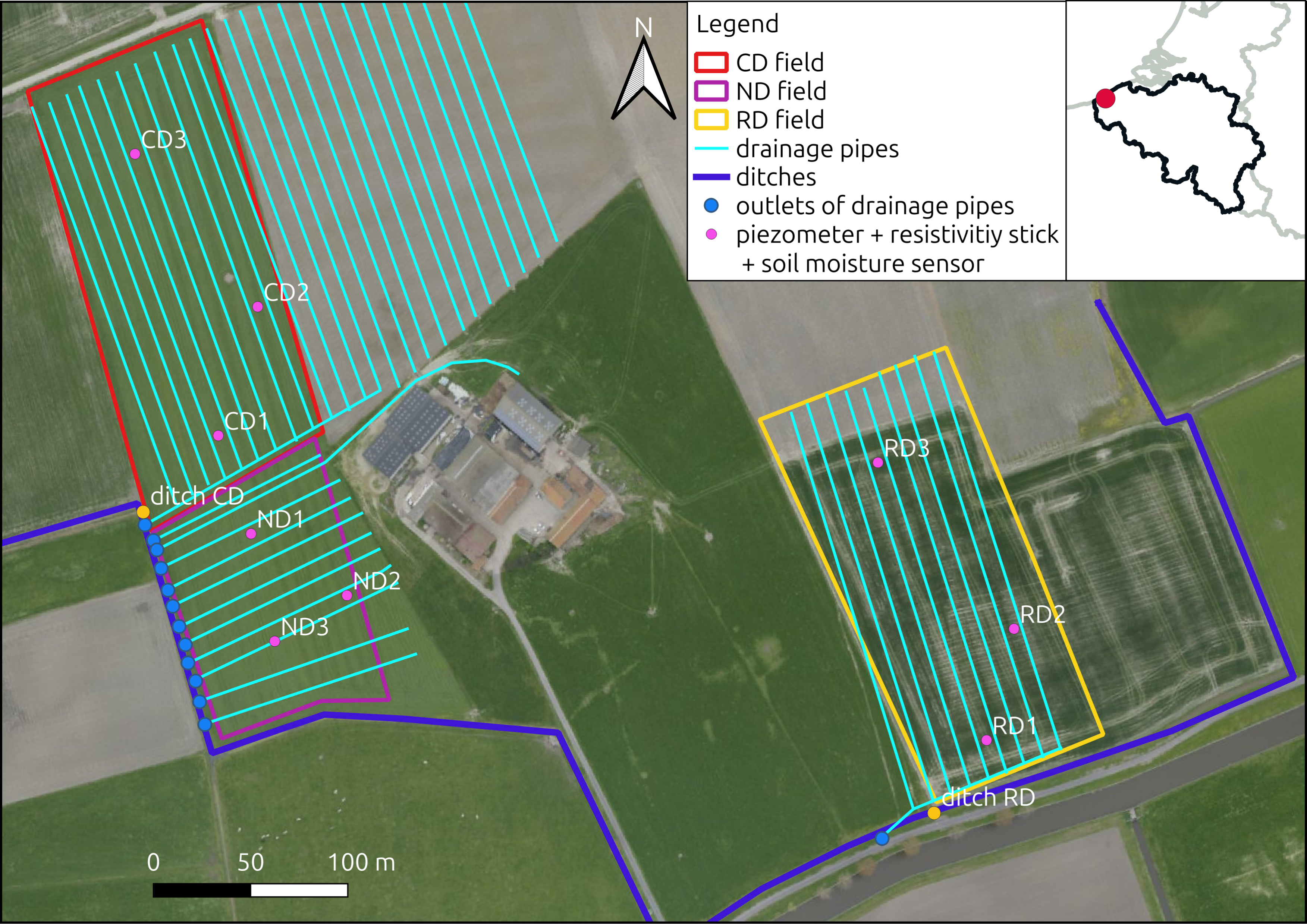
Overview of the experimental site in Middelkerke (Belgium) with three fields equipped (CD, RD and ND). In each field, three locations are monitored (e.g. RD1, RD2, RD3). The drainage system (PVC drains at about 0.9 m depth, spaced 8 m with an average slope of 0.1%) are visible in cyan. In the CD and RD field, the south–north drains are merged into a collector drain and brought to a control pit where an elbow can adjust the water table. Blue dots denote outlet of drainage pipes (or control pit) in the polder-managed ditch (dark blue). Masquer
Overview of the experimental site in Middelkerke (Belgium) with three fields equipped (CD, RD and ND). In each field, three locations are monitored (e.g. RD1, RD2, RD3). The drainage system (PVC drains at about 0.9 m depth, spaced 8 m with an ... Lire la suite
2.2. Instrumentation
Within each field, three locations were monitored. At each location, three piezometers were placed up to depths of 1.5, 2 and 3 m below surface from North to South, spaced 0.5 m (Figure 2). The piezometers have a screen on the bottom 0.5 m. The top 1 m part of the piezometer (from −0.5 to 0.5 m above surface) can be removed which enables us to bury the piezometer when large machinery for ploughing, sowing or harvesting needs to go on the field. Water samples from all piezometers were collected monthly and measured with a general lab conductivity meter and a Na+ specific sensor (LAQUAtwin-Na-11, Horiba, Japan). The deepest piezometer of each location (e.g. CD1-300) was equipped with a CTD diver (Van Essen Instruments, Waterloo, Canada) or a DL-CTD10 (Decentlab, Dübendorf, Switzerland) to measure pressure, temperature and electrical conductivity (EC). The pressure data were corrected for barometric pressure variations to obtain raw water heads. Given that the density of saline water is larger than the density of freshwater, the same pressure at the sensor can be linked to different heads of water above it. Hence, the raw water heads were then corrected to freshwater heads based on the electrical conductivity observed (e.g. Vandenbohede, Lebbe, et al., 2008). The difference between raw water heads and corrected freshwater heads was less than 0.015 m. From manual augering, different soil layers were identified from top to bottom: first an Ap layer used for agricultural activities, then a consolidated clay layer with traces of rust, then unconsolidated (unripened) clay (i.e. clay that was always under the water table, that never consolidated or ripened in unsaturated condition) were found. In some locations, peat layers were found. In addition to the piezometers, each location is also equipped with an ERT stick with 16 ring electrodes, spaced 0.15 m with the first electrode at 3.05 m depth and the last at 0.8 m depth below surface. The sticks in CD and RD fields have a diameter of 0.05 m, stainless steel electrodes rings internally connected. Spacers between rings are made of plastic and screw into each other. This modular design enables us to build a stick of the desired length. The sticks in the ND field are built around a bamboo stick of 0.015 m diameter. The electrodes are made with the last 0.3 m naked extremities of the cable (tinned copper) coiled and soldered on top of aluminium foil to increase contact area. This design, while less robust, is cheaper and similar data quality (reciprocal error, stacking error, contact resistances) is observed for both types of sticks. A Wenner sequence where potential electrodes are between the current electrodes, all four electrodes equally spaced was used. This sequence was acquired monthly with a Syscal Pro 120 (Iris Instrument, Orléans, France). A PRIME geoelectrical monitoring system (e.g. Chambers et al., 2022) was also used to monitor the sticks in CD1 and CD2 daily with the same sequence. Figure 2 shows the apparent electrical conductivity (ECa) derived from the ERT readings along the sticks. The ECa increases with depth and this increase is often associated with the presence of peat. Locations without peat in the first 3 m (like RD3) show a lower ECa value. Time-domain transmission soil moisture sensors (TMS-4, TOMST, Wild et al. 2019) were installed at depth of 0.15, 0.3 and 0.45 m at all CD and RD locations and in ND1. These sensors were also installed at 1, 1.5 and 2 m to measure soil temperature variation. Frequency domain electromagnetic induction (EMI) data were collected using a DUALEM-421S (Dualem Inc., Canada) that can measure up to 6 different coil configurations: PRP1.1 (perpendicular orientation with 1.1 m between transmitter and receiver coil), PRP2.1, PRP4.1, HCP1 (horizontal coplanar orientation), HCP2 and HCP4.
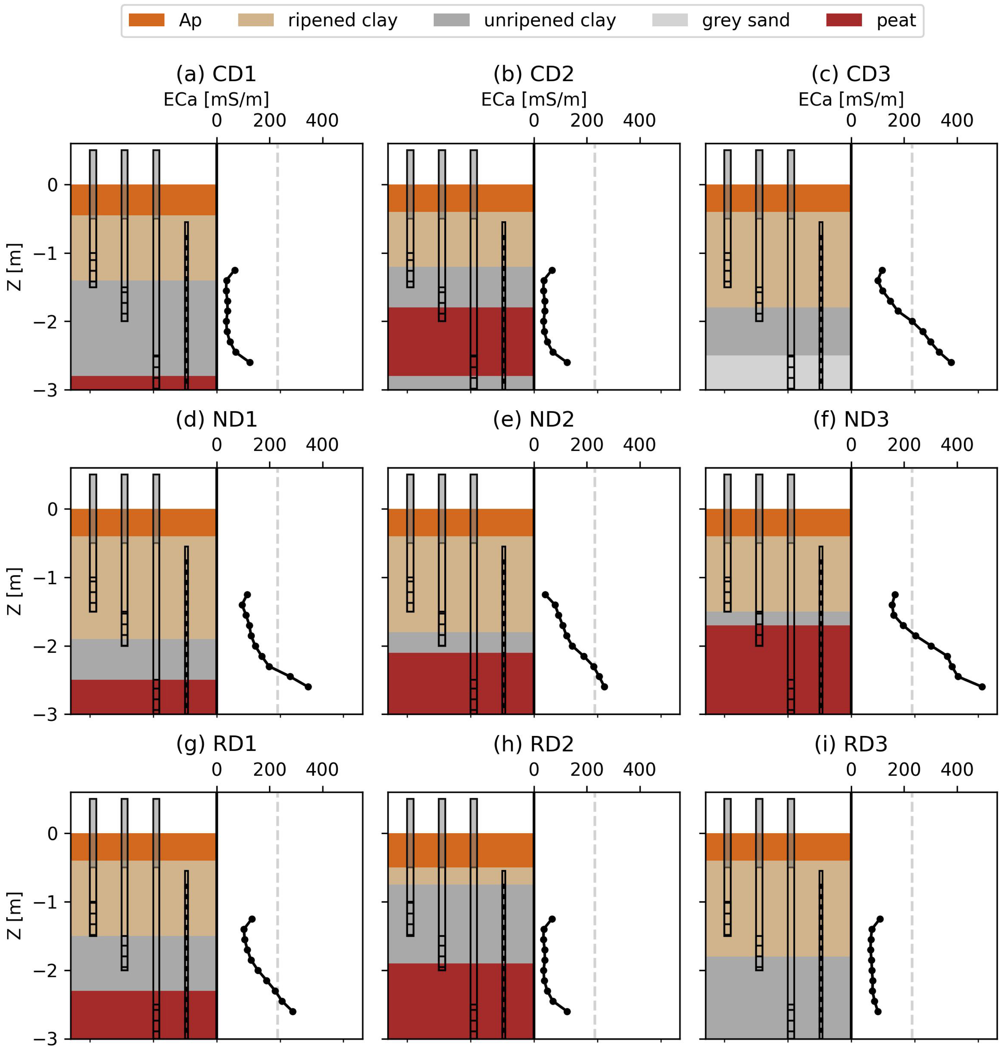
Each location is equipped with three piezometers with depths of 1.5, 2 and 3 m (with screen length of 0.5 m at the bottom of the piezometer). In addition, an ERT stick with 16 electrodes spaced of 0.15 m with first electrodes starting at 0.8 m depth is placed next to the piezometers. The different soil layers that have been observed while installing the piezometer are also shown. The raw ECa collected from the Wenner array is shown on the right of the profile (the depth is the midpoint of the quadrupole). The dashed vertical grey line shows the 230 mS/m threshold. Masquer
Each location is equipped with three piezometers with depths of 1.5, 2 and 3 m (with screen length of 0.5 m at the bottom of the piezometer). In addition, an ERT stick with 16 electrodes spaced of 0.15 m with ... Lire la suite
2.3. Data processing
EC and ECa from ERT stick values presented in this work were temperature corrected to 12 °C (average groundwater temperature of the field) following: EC12 = EC/(1 + 0.02 × (T − 12)) (Ma et al., 2011) where T is the temperature in degC. Electrical resistivity data from surface arrays were processed using ResIPy (v3.4.5, Blanchy, Saneiyan, et al. 2020, Binley and Slater 2020). Quadrupoles were kept if the current injected was larger than 1 mA, stacking error smaller than 10% and reciprocal error smaller than 20%. The data were inverted on an axis-symmetrical mesh (resistivity can vary with depth and away from the stick). The axis-symmetrical constraint was imposed on a 3D mesh by defining rings of parameters, similar to Ronczka et al. (2020). A difference inversion (reg_mode=2) scheme was used (LaBrecque and Yang, 2001). The inversions converged in less than 5 iterations, reaching a final weighted root mean squared close to 1. While the inversions were successful, they tended to oversmooth the fresh–saline water boundary, hindering the seasonal variations that could be observed in the raw ECa. Hence, we decided to further present the resistivity data as apparent electrical conductivity by selecting all quadrupoles where all electrodes were spaced by two electrode spacing. The depth assigned to the ECa of a quadrupole is the midpoint of the quadrupole. The EMI data processing included georeferencing and drift correction following Hanssens (2020). The obtained values are also displayed in ECa in mS/m. Statistical comparison between fields was done using independent t-tests with scipy v1.14.5 (Virtanen et al., 2020). For each t-test the values of three locations (at a given depth and time) were compared between the field in controlled drainage (CD or RD) and the reference field (ND). Significant differences were established when the p-valuewas below 0.05.
2.4. Management
Two different drainage management methods were applied on the fields: controlled drainage and regular drainage. In controlled drainage, the groundwater table was managed by adjusting a pipe after the elbow connected to the collector drain in the CD and RD field (Figure 3). In regular drainage, the pipes were open completely, allowing the free drainage. In 2022, all fields were in regular drainage representing a reference situation (although not all fields had the same crops). In 2023, CD field was in controlled drainage (+0.2 m from drain level at outlet or 0.7 m from the surface) while RD and ND were in regular drainage. In 2024, CD and RD were in controlled drainage (+0.2 m from drain levels at outlet). The years 2023 and 2024 were wet and we did not raise the water level more than 0.2 m as the farmer did not want to risk part of the field to be flooded, damaging crop growth. The water level in the field in controlled drainage was occasionally lowered to drain level during field operations (sowing and harvesting mainly).
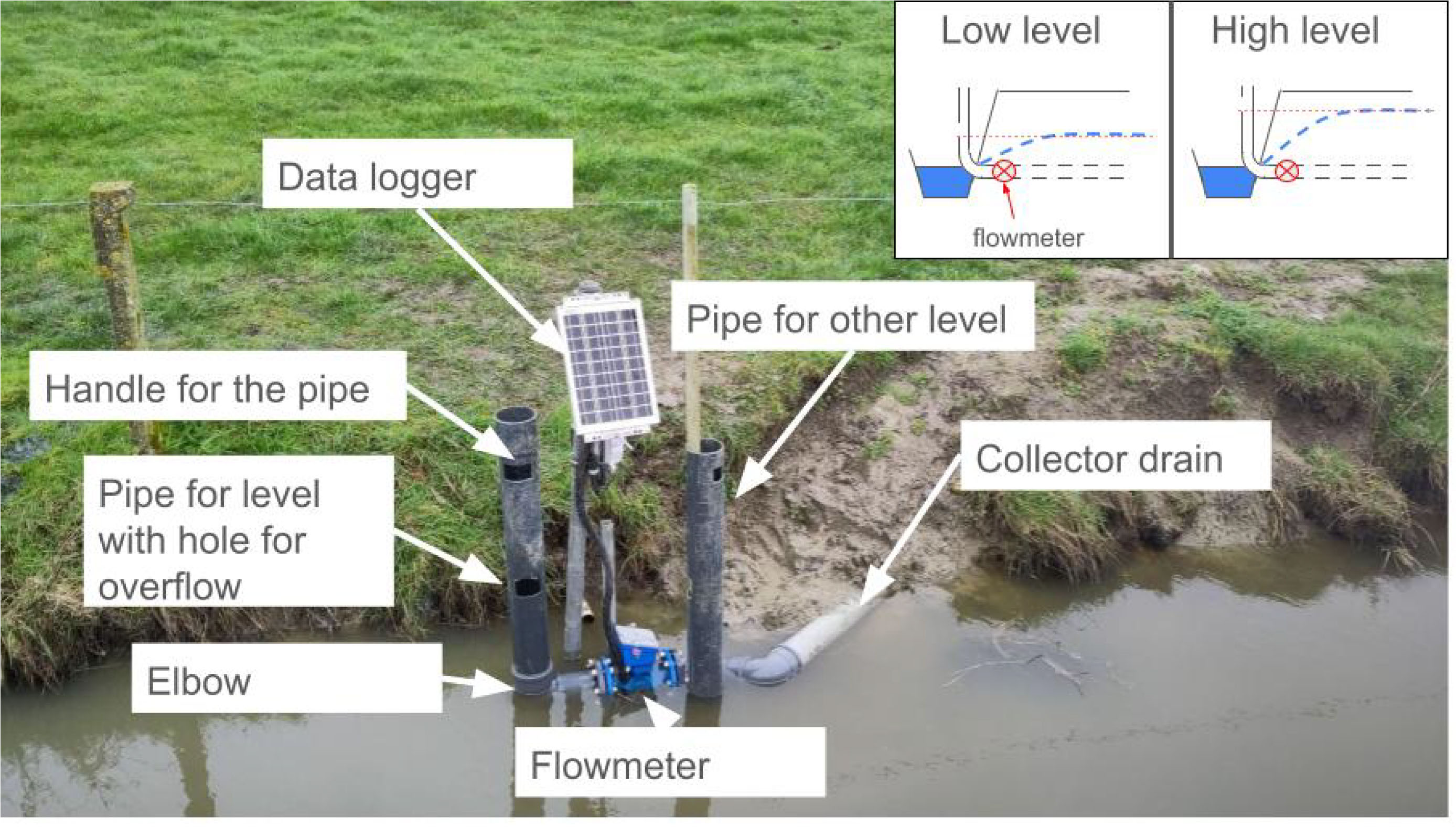
Controlled drainage system located in the RD field with the collector drain coming from the field going through the flowmeter, then the elbow on top of which a vertical pipe section with holes to a defined height is placed to apply the desired water level. Usually, this setup is placed in a control pit within the field to not block the waterways.
3. Results
3.1. Hydrology
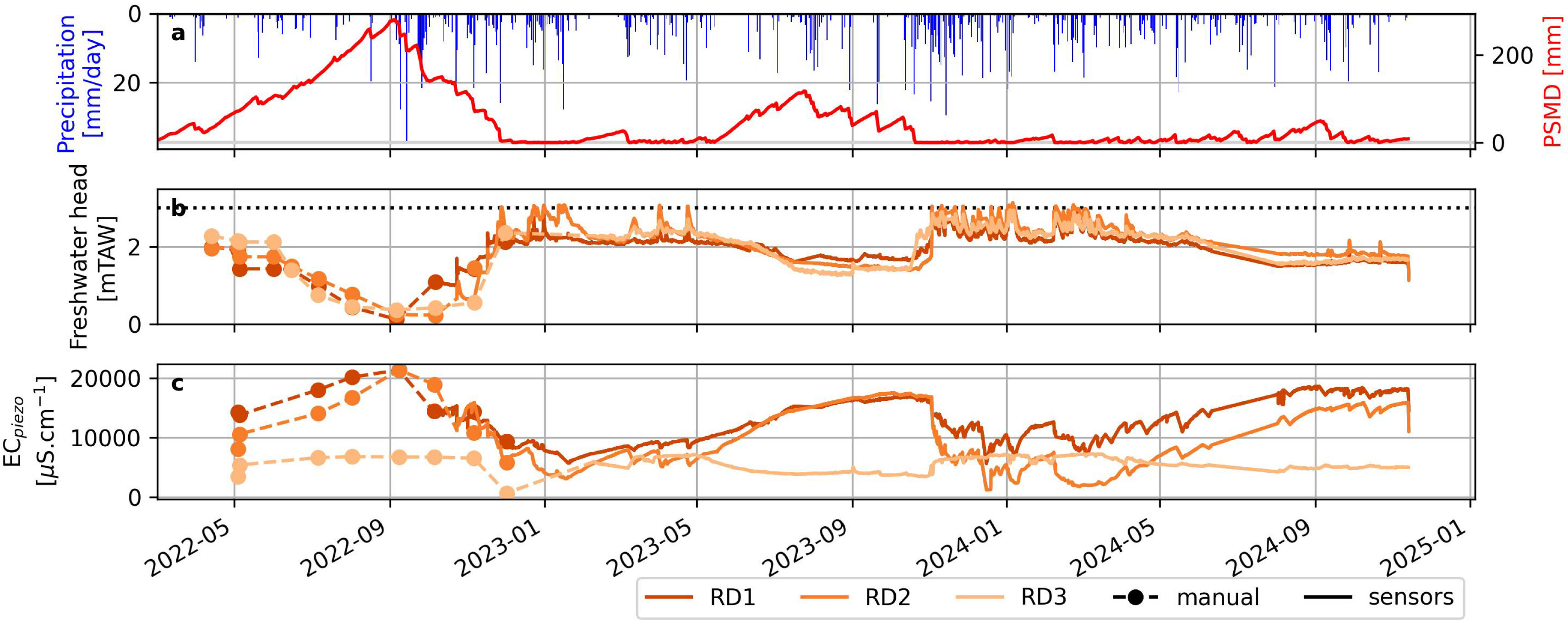
Figure 4 shows the evolution of the several variables for selected locations (CD2, RD2, ND2). Data from all locations are available in an interactive dashboard (see data availability section). The year 2022 was driest, with a large PSMD peak of 280 mm and was 2024 the wettest (Figure 4a). NDVI data shows the evolution of the crops. In 2022 and 2023, different crops were grown in CD & ND and RD fields (Figure 4b), followed by grass as cover crop in 2023 and 2024. The limited precipitation of 2022 and the larger water uptake from the grass in RD explain the larger decrease in groundwater observed for RD. Figure 4c shows the applied drainage depth for each field. Figure 4d shows the cumulative discharge from the drains divided by the drained area of each field. Note that the flowmeter in RD was only placed in autumn 2023. Drainage mostly occurs between September and January, but during the summer there was also a drainage flux in the ND field in 2023. This summer drainage is mostly due to intense summer precipitation events and amounts to 33 (2023) and 44 mm (2024) per year. The soil moisture (Figure 4e) in the fields decreases during summer months (up to 0.3 v/v) and recovers during winter (up to 0.4 v/v). Differences in soil moisture can be observed between the fields. For instance in June 2023, CD and RD fields show larger moisture content than the ND field. However, when all three locations of the fields are considered, this difference is not significant. In May 2024, the soil moisture content in the RD field was significantly larger than the CD or ND fields. The freshwater heads followed the expected pattern. They decreased during summer when there was insufficient precipitation to recharge the aquifer and uptake from the growing crops. During winter months there was a precipitation surplus that recharges groundwater up to drainage level. The water table in the field was often higher than the water table in the ditch but can also go below (e.g. in 2022 in the RD field). Significant differences in freshwater heads between the fields were observed in September 2022 (CD higher than RD), June 2023 (CD and RD lower than ND) and November 2023 (RD lower than ND). The increment of 0.2 m in controlled drainage fields was observed during winter months, but vanished after a month. The summer decrease of the water table was accompanied by an increase in the electrical conductivity of the water in the piezometer (ECpiezo)—here used as a proxy for salinity—. However, a lower water table does not always involve a larger salinity. In 2022, for instance, the water table drops much slower in CD2 than in RD2, but we recorded a large increase in salinity in both wells.
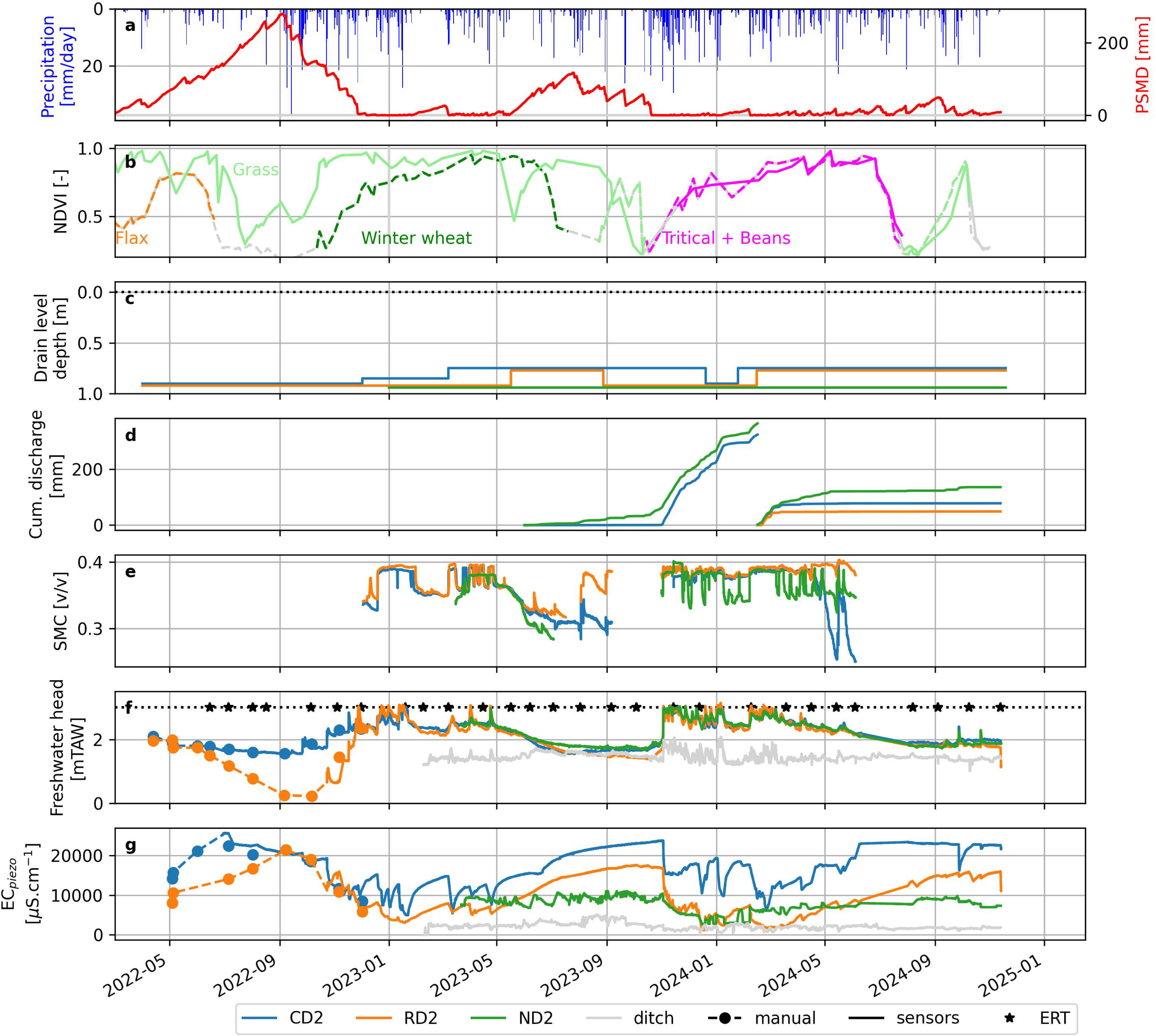
Three year time series showing: (a) daily precipitation and potential soil moisture deficit (i.e. cumulated potential evapotranspiration–precipitation), (b) normalised difference vegetation index (NDVI) obtained from remote sensing showing the crops in CD & ND (dashed line) and RD (solid line) fields, (c) water level imposed in the control pits, (d) cumulative yearly discharged observed (reset to 0 on 1st March), (e) volumetric soil moisture content at 0.3 m depth (SMC), (f) freshwater heads and (g) electrical conductivity of the water inside the piezometers. These time-series combined manual (dots) and sensor (line) data for one location per field (CD2, RD2, ND2) as well as for the ditch close to the RD outlet. Acquisition days of electrical resistivity tomography (ERT) are denoted by stars in (f). Masquer
Three year time series showing: (a) daily precipitation and potential soil moisture deficit (i.e. cumulated potential evapotranspiration–precipitation), (b) normalised difference vegetation index (NDVI) obtained from remote sensing showing the crops in CD & ND (dashed line) and RD (solid line) fields, ... Lire la suite
3.2. Spatial heterogeneity
EMI mapping and the micro-topography map demonstrated the field displays significant spatial heterogeneity. Figure 5 shows the digital elevation model (DOV), revealing microtopographical variations related to buried landforms and past land use. Figure 5b shows the map of the EMI on top of the elevation model. Low-lying areas are generally associated with a higher ECa. EMI data also reveal the presence of less conductive linear features in the RD field, with RD3 being placed just in the middle of one of these. These are likely related to past hydrological structures (palaeochannels) that have been filled in with less conductive (sandy) deposits. We hypothesize that this palaeochannel system continues in the CD field at CD1, and then extends further north-west. Augerings conducted during piezometer installation confirm that RD3 and CD1 are more sandy at depth.
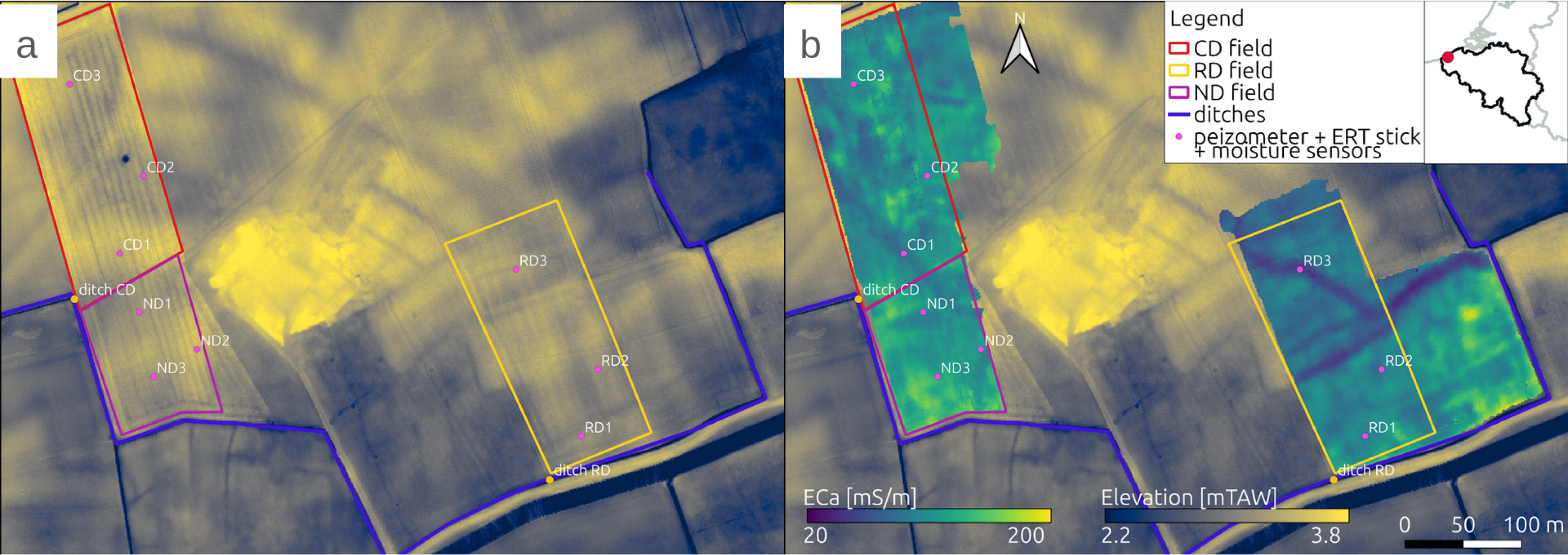
(a) Microtopography of the fields around the farm derived from the digital elevation model from Databank Ondergrond Vlaanderen (DOV). (b) Electromagnetic induction map (EMI) showing the apparent electrical conductivity for the HCP 1 m configuration of the DUALEM-421S.
Figure 6 shows the soil moisture content, freshwater head and electrical conductivity of the groundwater for the piezometer RD3 installed at 3 m depth in the RD field. This point is located in the sandy channel detected by the EMI soil scan. The groundwater salinity in RD3 time series follows a different pattern than the one in RD1 and RD2. While the freshwater head decreases for all piezometers, the electrical conductivity of the groundwater in RD3 does not increase as in RD1 or RD2. The sandy channel probably stores more fresh water since precipitation infiltrates more easily in that soil texture and also lateral flow can occur. The effect of this natural freshwater barrier formed by the sandy palaeochannel can be well observed in the EMI map (Figure 5). The part of the field South of the channel shows a higher ECa compared to the part right above the channel. In the CD field, CD1 also shows a lower EC compared to CD2 or CD3, possibly because it is also located in a backfilled sandy channel.
(a) Rainfall and potential soil moisture deficit (PSMD = cumulated potential evapotranspiration—precipitation). (b) Freshwater head and (c) electrical conductivity in the 3 m piezometer.
One of the goals of controlled drainage is to store more freshwater than in the case of regular drainage. Figure 7 proposes an estimation of the repartition of the precipitation into different fluxes. It shows that most of the drainage and the infiltration occurs during winter months. Little drainage occurs during summer, mainly during intense precipitation events. We previously showed that the water from intense precipitation events is drained out of the field into regular drainage (ND field), while controlled drainage (CD field) retains this water so that it remains available to the crop later in the season. This explains the difference in total drainage observed in 2023 and 2024 between CD and ND. 33 (2023) and 44 mm (2024) of water was buffered in the controlled drainage field (CD). This amount, while representing less than 10% of the total water drained during a season, is the equivalent of one irrigation event.
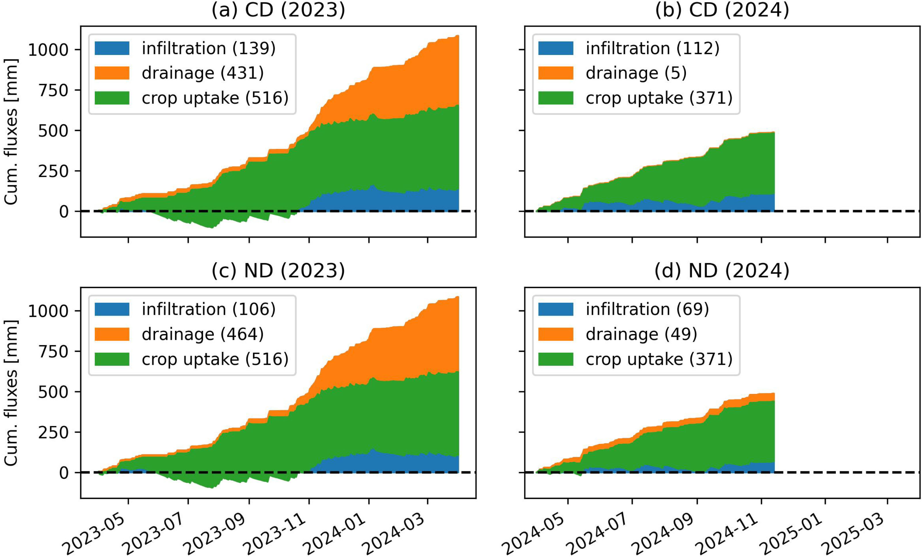
Evolution of the amount of precipitation distributed among drainage, infiltration and crop uptake flux. Crop uptake is the potential evapotranspiration, and as such, is certainly overestimated. Drainage flux is measured with the flowmeters. Infiltration is what remains. When the total flux goes below the dashed line (becomes negative), it means the precipitation is not sufficient and groundwater is used to support crop growth. Numbers in parentheses represent mm of precipitation.
3.3. Electrical resistivity
Based on the monthly observed ECa values along the sticks, the EC of the water in the piezometer, and the lithology (Figure 2), a threshold of 230 mS/m was estimated to delimit the fresh–saline water boundary. This threshold is based on the median between all times and locations of the middle of the range of ECa observed in the saturated zone. Data from CTD divers shows that the EC of the water below this threshold is often larger than 10,000 μS/cm and up to 25,000 μS/cm during summer peak (Figures 4, 6). Figure 8 shows the evolution of this threshold in time. We defined everything below the threshold as saline and everything above it as fresh water. The top of the freshwater part represents the water table. This figure depicts the evolution of the thickness of the freshwater lens throughout three growing seasons. During summer, the freshwater lens is increasingly exploited by the crop. In the summer of 2023 and in CD2, the freshwater lens was almost completely depleted. During summer, the fresh–saline water boundary moves upward, possibly due to the reduction of the vertical freshwater head. Note that RD3 does not show ECa values above 230 mS/m. It behaves differently, since it is located in a sandy area within a palaeochannel (see Figure 5).
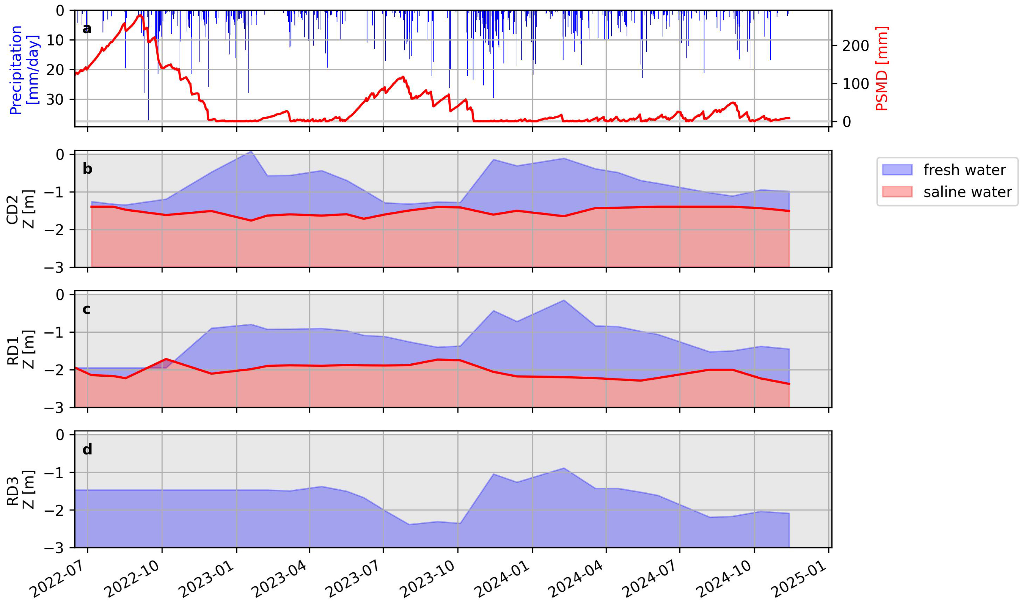
(a) Rainfall and potential soil moisture deficit (PSMD = cumulated potential evapotranspiration–precipitation). (b–d) Estimations of the thickness of the freshwater lens based on a 230 mS/m threshold applied on the apparent electrical conductivity from the ERT sticks. The time resolution of this figure was adapted to follow the resolution of the ERT surveys that were carried out every month (precise dates in Figure 4c).
To separate the static effect of the material electrical conductivity from the dynamic effect of the pore water electrical conductivity, time-lapse differences are shown in Figure 9. Differences in ECa are driven by soil moisture content above the water table and by change in salinity below the water table. In the unsaturated zone, soil moisture dynamics dominate the signal, although simultaneously also changes in pore water concentration might be occurring. There is an increase in ECa below the water table in both CD2 and RD1 during the summer of 2023, which aligns well with the trend of the threshold shown above (Figure 8). In contrast, the decrease in soil moisture in RD1 during summer 2022 led to a decrease in ECa. The dynamic of RD3 (piezometer located in the sandy channel) is clearly different from CD2 or RD1 with lower magnitude of change and no increase in ECa below the water level during summer time. A slight increase in ECa above the water table can also be observed during summer time in RD1, possibly explained by capillary rise of saline water in the unsaturated zone. However, we acknowledge that more work is needed to test this hypothesis.
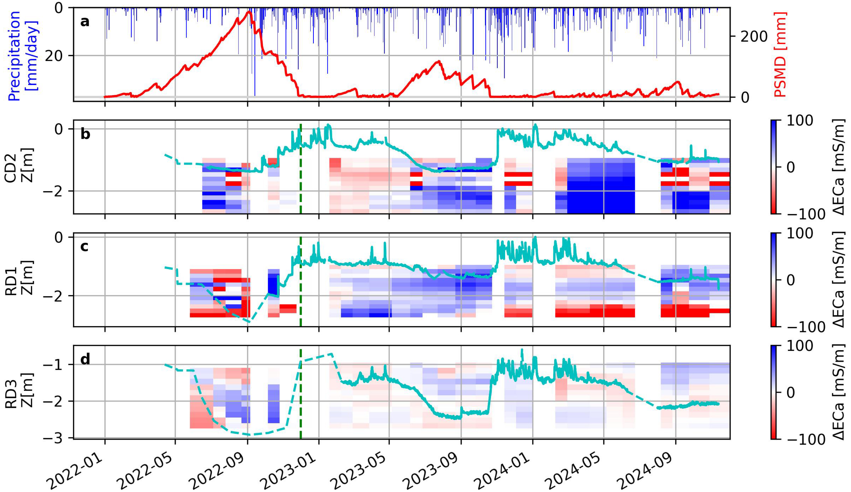
(a) Rainfall and potential soil moisture deficit (PSMD = cumulated potential evapotranspiration—precipitation). (b) Difference in apparent electrical conductivity for three locations with the water table in cyan. Differences are computed compared to a “wet reference” survey denoted by the vertical dashed green line. Increase in ECa can be associated with increase in saturation above the water table and increase in salinity below the water table.
4. Discussion
The effectiveness of controlled drainage depends on factors such as, the distribution of the precipitation, as demonstrated by several modelling studies (e.g. Rodriguez et al., 2024). Mainly in years with summer droughts, agronomic benefits can be expected, since controlled drainage assures more of the precipitation in spring and summer is turned into soil water storage, instead of drainage. Among the three monitoring years at our experimental site, only 2022 was a “dry year”. However, in 2022, all three fields were still under regular drainage. Different crops were grown in the RD (grass) and CD (flax) field, which had a large effect on the groundwater table (Figure 4). In the years 2023 and 2024, controlled drainage was implemented, but those years were very wet. This abundance of summer precipitation resulted in a lack of significant differences in yield between the controlled drainage fields and the regular drainage, since no drought stress was occurring in either of them. Nonetheless, Youssef et al. (2023) also found little to no increase in corn yield with controlled drainage based on the 55 site-years data from several fields in the US. Similarly, a world-wide meta-analysis of Wang et al. (2020) found that controlled drainage increases yield by 0.11% on average. Controlled drainage also has the potential to increase the retention time of nutrients and fertilizer in the field. While investigating this was beyond the scope of this work, this could equally impact crop health (Castellano et al., 2019).
While we saw a pronounced seasonal effect on the fresh–saline water interface, we could not see a clear difference between controlled and regular drainage. We expected that the combined low water level in the ditch surrounding the field (due to the polder water board) and the higher head in the field (due to controlled drainage) would have encouraged saline water to flow from the field to the ditch. However, this process can be slow and longer term studies will be needed to observe this effect.
From piezometer data, saline water can be found at various depths within the same field. The reason for the differing data in several piezometers in the same field became clearer with the help of geophysics (EMI map in Figure 5). Similarly, while the EC of the water in the piezometer provides a good proxy for the depth of the saline water, the addition of the ERT sticks to locate the fresh–saline water boundary in the bulk soil (Figure 8) is unique. Overall, the heterogeneity of the agricultural field, especially the presence of the sandy channel and the presence of peat layers with higher hydraulic conductivity than the clay layers may have a large effect on the field hydrology, maybe even larger than the effect of controlled drainage. Such structures are not uncommon in polder areas, whether their origin is natural or artificial (deviation of water course or merging of agricultural parcels).
The 230 mS/m threshold is a relatively simple approach to delineate the fresh-saltwater interface, but we also observed that the higher ECa values were co-located with the presence of peat (Figure 2). Hence, one can wonder how to distinguish the static contribution of the soil materials from the contribution of the pore water EC. Petrophysical models (e.g. Archie, 1942 or Waxman and Smits, 1968) could be applied per material. However, given the different support volumes of the ERT sticks and the piezometer, we choose to not explore a more advanced approach in this manuscript. Instead, we separate the static effect of the material electrical conductivity from the dynamic effect of the pore water electrical conductivity by looking at time-lapse differences (Figure 9).
Typically resistivity readings obtained from ERT sticks are inverted to estimate the exact depth of the fresh–saline interface (e.g. Ronczka et al., 2020). For this work, we choose not to present the inverted results, but to work with the raw temperature corrected ECa instead. While the axis-symmetrical inversions of the ERT sticks converged well and provided meaningful depth-specific insights into the lithology, the evolution of the fresh–saline boundary established based on the 230 mS/m threshold was lost during the smoothness-constrained inversion. This can be partly explained by the imposed constraints. We hypothesize that, during the summer, the greater extent of the unsaturated zone (more resistive) and the increase in salinity in the deeper layer (less resistive), can compensate and be smoothed out during the inversion process. The inclusion of the measured water table as a sharp boundary could potentially help to solve the issue even if the capillary zone in clay soil is likely a smooth transition between saturated and unsaturated zone. The effect of the unsaturated zone on the inversion was already mentioned by Velstra et al. (2011). Our higher time-resolution 1D data make them more sensitive to this effect. However, in our setup, the measurement of vertical quadrupoles along the ERT sticks enables us to locate the depth of the fresh–saline water interface accurately compared to a setup with only surface electrodes.
5. Conclusion
The effect of controlled drainage on the seasonal dynamics was minimal in our study, probably due to the wet conditions in comparing controlled and regular drainage. Controlled drainage was still able to buffer intense precipitation events (up to 44 mm in 2024) which could have been beneficial to crops should a long dry period have occurred subsequently. The geophysical measurements (EMI and ERT) proved useful in unravelling the field-scale spatial heterogeneity and helped in the interpretation of traditional hydrological point sensors. Field heterogeneity, including human-induced and natural structures, play an important role in the hydrological functioning of the studied parcels. This is a situation which is likely to occur in many polder landscapes and was revealed thanks to EMI measurements. The evolution of the raw ECa values from the ERT sticks enable us to follow the freshwater lens thickness and observe how, as the freshwater lens decreases during summer, the saline groundwater tends to rise up. However, no significant effect of controlled drainage on the evolution of the fresh–saline water interface was observed. While, additional information from piezometers and augering is needed to correctly interpret the geophysical data, the ERT and EMI techniques offer invaluable spatial and temporal information at relevant scales to the study of the fresh–saline water interface for agronomical applications.
Data and code availability
All the data and code used in this study is available at https://github.com/op-peil/paper-setup (Blanchy, Everaert, et al., 2025).
Declaration of interests
The authors do not work for, advise, own shares in, or receive funds from any organization that could benefit from this article, and have declared no affiliations other than their research organizations.
Authorship statement (CreDIT)
Conceptualization: GB, SG, TH, FN, PS, DH; formal analysis: GB, ER; data curation: GB, ER, BE, AM, DC, PS; writing - original draft: GB; writing - review and editing: All authors; project administration: GB, SG, TH, FN, PS, DH.
Funding
GB is a Research Fellow of the Fonds de la Recherche Scientifique—FNRS (CR: 1.B.044.22F). The experimental site and the majority of the hydrological data were collected in close collaboration with the OP-PEIL project (VLAIO HBC.2020.3159) funded by the Flemish Government.
Acknowledgments
We would like to thank Valentijn Van Parijs for doing most of the EMI data collection and Dirk Demeyere for letting us run this experiment in his fields.