CC-BY 4.0
1. Introduction
The Critical Zone (CZ) is the outermost layer of the Earth’s crust, extending from the bedrock to the uppermost layer of the vegetation canopy. Here, interactions between bedrock, soil, water, air and living organisms influence the formation of landscapes and ecosystems (Dumont et al., 2022; Giardino and Houser, 2015; Parsekian, Singha, et al., 2015). To address environmental challenges and manage natural resources, understanding structure, properties, and processes within the CZ is highly important. This understanding is tied to the different components of the CZ, consequently the investigation takes place at different scales, ranging from the microbial to the catchment scale. A key concern is climate change and loss of arable land. To ensure the ability to feed future generations, we must increase food production while using fewer natural resources. The impact of agriculture on the soil-plant continuum is significant and because it’s a very dynamic and heterogeneous system, which makes it hard to study and monitor. There is a growing interest in non-invasively investigation techniques measuring at field-to-plot scale, as short-term and site-specific management approaches become increasingly prevalent in modern precision agriculture (Pasquel et al., 2022). This highlights the need for the development of non-destructive, high-resolution methods for the understanding of small-scale soil ecosystem processes in the CZ.
The investigation of the soil-plant continuum at a field-to-plot scale using geophysical measurement techniques such as ground penetrating radar (GPR) has become increasingly popular in the last decade because of its high-resolution capability and direct relationship to soil water content (SWC) (e.g., Parsekian, Singha, et al., 2015; Klotzsche, Jonard, et al., 2018; Huisman et al., 2003; Garré et al., 2021). GPR is an electromagnetic (EM) method that records the propagation of EM waves through the subsurface, influenced by the dielectric properties of the soil components. The propagation of EM waves allows the calculation of the relative dielectric permittivity 𝜀r of the soil. The SWC can be derived using empirical or petrophysical mixing models using 𝜀r (Steelman and Endres, 2011). Among near-surface geophysical methods, GPR can achieve high spatial resolution, providing detailed images of subsurface structures that exceed the resolution capabilities of other methods. Next to the 𝜀r, the electrical conductivity 𝜎 of the different soil components affect the EM waves, especially amplitudes. Generally, an increased 𝜎 attenuates the GPR signal (Jol, 2009).
When investigating the soil-plant continuum of fine root systems (root diameter < 2 mm) is especially challenging. First, accurately identifying individual roots of fine root systems is particularly difficult, caused by a combination of technical and physical limitations. When the diameter of the roots is smaller than the wavelength of the GPR signal, individual roots cannot be detected, only root zones containing a certain number of roots can most likely be detected. Additionally, crop root systems grow in dense clusters, which can cause an overlapping or combination of the GPR signals of the individual roots.
Second, the presence of small-scale soil heterogeneities and fine root systems creates non-uniqueness within the GPR signal. These heterogeneities affect processes such as infiltration, soil water depletion, and root growth, making it difficult to distinguish between soil, root zones, and pore filling just based on GPR signals (e.g., SWC, fertilizer). The biological, hydrological, and chemical processes that occur within the soil-plant continuum are highly dynamic and influenced by a variety of factors. These range from atmospheric weather conditions, soil physical and chemical properties, nutrients, microorganisms to root architecture and agricultural management practices. These two points could be addressed by applying high-frequency GPR system, however this brings us to the third issue. When using high frequencies in the field, a high attenuation and scattering of the EM waves occurs, which limits the penetration depth. As a result, mapping and detecting fine root systems in the field using GPR remains a significant challenge.
Several studies have been conducted to investigate the soil-plant continuum of plants with fine root systems using GPR measurement techniques (Wijewardana and Galagedara, 2010; Liu, Dong and Leskovar, 2016; Liu, Dong, Xue, et al., 2017; Delgado et al., 2017; Klotzsche, Lärm, et al., 2019; Lärm, Bauer, van der Kruk, et al., 2024). One of the earlier works by Wijewardana and Galagedara (2010), which used surface GPR to estimate the spatial and temporal distributions of SWC in raised beds cropped with vegetables, with a particular focus on understanding the effects of irrigation on SWC patterns. Liu, Dong, Xue, et al. (2017) linked 1600 MHz GPR images to root diameter and biomass measured from soil cores for winter wheat and energy cane grown in different soil types. In a laboratory setting, Parsekian, Slater, et al. (2012) successfully detected roots as small as 2 mm in diameter using 1600 MHz antennas.
To study soil-plant continuum processes, time-lapse information can be highly beneficial. One of the first longer-term time-lapse GPR dataset was acquired at the field minirhizotron (MR) facilities in Selhausen, Germany. These platforms feature horizontal rhizotubes at multiple depths, installed in two contrasting soil types, to assess the impact of, e.g., changing atmospheric conditions and agricultural management practices (Lärm, Bauer, Hermes, et al., 2023). As demonstrated by Klotzsche, Lärm, et al. (2019) and Lärm, Bauer, van der Kruk, et al. (2024), who used longer-term time-lapse horizontal crosshole GPR measurements to monitor the crop-root systems over various growing seasons (winter wheat and maize), it was observed that crops with a higher crop row distance, such as maize, can influence the variability (horizontally and vertically) of the 𝜀r and, consequently, the SWC. In contrast, wheat has been observed to exhibit a more homogeneous effect on the GPR data. Lärm, Bauer, van der Kruk, et al. (ibid.) were able, to qualify the influence of maize roots on the GPR signal throughout the vegetation period using statistical methods like spatial and temporal permittivity variability analysis. However, to date, a direct and quantitative relationship and possible error estimates between the GPR signal and root presence, actual water present in the soil, roots, or the above-ground shoot (connected to stem flow and infiltration processes) and soil nutrients have not been established. Additionally, the setup of the field MR facilities itself posed some issues, e.g., the overlapping of the critically refracted air wave and the direct ground wave when using standard processing techniques (Klotzsche, Lärm, et al., 2019). This caused lower permittivity values than present in the soil within the uppermost depths, especially during dry conditions.
Despite these advances in monitoring spatial and temporal variation in soil-plant continuum using GPR, a fundamental obstacle remains: the lack of quantitative knowledge of the permittivity of agricultural roots. This complicates distinguishing roots from surrounding soil and additionally complicates establishing models relating GPR signals to actual SWC, root presence, or root related processes. Estimating the permittivity of roots is additionally not straightforward, it can vary with multiple factors, such as, crop type, root type, age/physiological status, water content of the surrounding soil and fertilizer applications. Quantitative values are abundant in literature. Attia Al Hagrey (2007) listed permittivities for wet and dry cellulose, but these values are not quite applicable for crop/maize roots. This is because they are not entirely made up of cellulose. Miao et al. (2015) reported that the cellulose content of maize roots varies in maize roots depending on fertilizer applications, ranging from 14.6 to 33.0%. Furthermore, we cannot equally compare tree roots and crop roots, since trees are perennial and crops are annual plants. Roumet et al. (2006) found several important differences in the root traits of annuals and perennials, which were key to their ability to take in resources and conserve them. Perennials exhibited higher specific root length, root nitrogen concentration and mycorrhizal colonization, but lower root tissue density than the annuals. According to Coners and Leuschner (2005) the surface area of fine roots (less than 2 mm) is the main factor in determining how much water and nutrients plants take up.
The roots not only affect the soil water content in the soil-plant continuum, but also change the water content in close proximity to the roots. For example, mucilage increases the water holding capacity and the soil pore structure can be permanently altered by the roots, creating preferential pathways (Angers and Caron, 1998; Carminati et al., 2011; Gerke and Kuchenbuch, 2007; Kodešová et al., 2006). These small-scale changes in SWC and linked gradients towards the roots cannot be modelled with gprMax, especially when the grid size is 0.01 m.
In this study, we investigate the potential for differentiating between soil water and roots using horizontal crosshole GPR data applying synthetic forward modeling. It is crucial to derive the available water content in the soil without the influence of water-filled roots from GPR measurements, to reduce uncertainties for management decisions. Therefore, as a first step, we explore the effect of calculating the SWC using conventional petrophysical relationships in which we can consider the various soil components. As a preliminary step, we incorporated a root contribution into the petrophysical relationship and examined the impact of this root component on the GPR-derived SWC. Furthermore, we employ synthetic forward modeling with the open-source electromagnetic simulation software gprMax (Warren et al., 2016) considering in the modeling domain soil, root and shoot information to address questions about above- and below-ground effects. The enhance the understanding a realistic model, root distributions in a soil associated with maize crops, root volume fraction (RVF) data derived from trench wall root count measurements acquired for maize (Klotzsche, Lärm, et al., 2019; Morandage et al., 2021) additionally to the soil information. As in previous studies, the standard first arrival time picking of the GPR EM waves were used to derive the 𝜀r of the soil and, consequently, the SWC of the soil-plant continuum. Synthetic models can help to understand processes of the real world and their effects measurement scenarios.
2. Materials and methods
2.1. Measurement platform and GPR data acquisition
To investigate the different influences on the GPR signal, we used the field MR facilities as a template for the setup of our synthetic forward model (Figure 1). The two facilities were part of the TERENO (TERrestrial ENvironmental Observatories) Eifel/Lower Rhine observatory, located near Selhausen (50°52′N, 6°27′E) and the setup was mirrored in two different soil types. The first was the upper terrace minirhizotron facility (RUT), which was situated in soil classified as Orthic Luvisol with a high stone content (>50%) according to the World Reference Base for Soil Resources (IUSS Working Group WRB, 2007). The second was the lower terrace minirhizotron facility (RLT), which is located in soil classified as Cutanic Luvisol (Ruptic, Siltic) according to the World Reference Base for Soil Resources (ibid.). Both facilities featured 7 m-long horizontal rhizotubes installed at various depths (0.1, 0.2, 0.4, 0.6, 0.8 and 1.2 m), enabling crosshole GPR measurements and acquisition of root imaging using minirhizotron camera systems. Each facility was divided into three replicas (plots) and each plot hosted three horizontal rhizotube per depth, with a horizontal spacing of 0.75 m. Between the different depths a horizontal offset was present to prevent an interference of the rhizotubes with root growth (Figure 1). Above the subsurface the plots operated as regular agricultural fields, where crop management was performed in compliance with regional standards. The crops were sown perpendicular to the rhizotubes. For a detailed description of the construction of the facility we refer to Cai et al. (2016) and for a detailed description of the data acquisition and analysis we refer to Lärm, Bauer, Hermes, et al. (2023). To acquire crosshole GPR measurements within the field MR facilities standardly a 200 MHz PulseEKKO borehole system (Sensors and Software, Canada) was utilized. As an acquisition setup zero-offset profiling (ZOP) was used, whereby the transmitter (Tx) and receiver (Rx) antennae were placed in neighboring rhizotubes and moved simultaneously in parallel positions along the rhizotubes with a step size of 0.05 m.
Exemplary plot within the field MR facilities with the schematic illustration of zero-offset profiling using a 200 MHz crosshole GPR measurement system.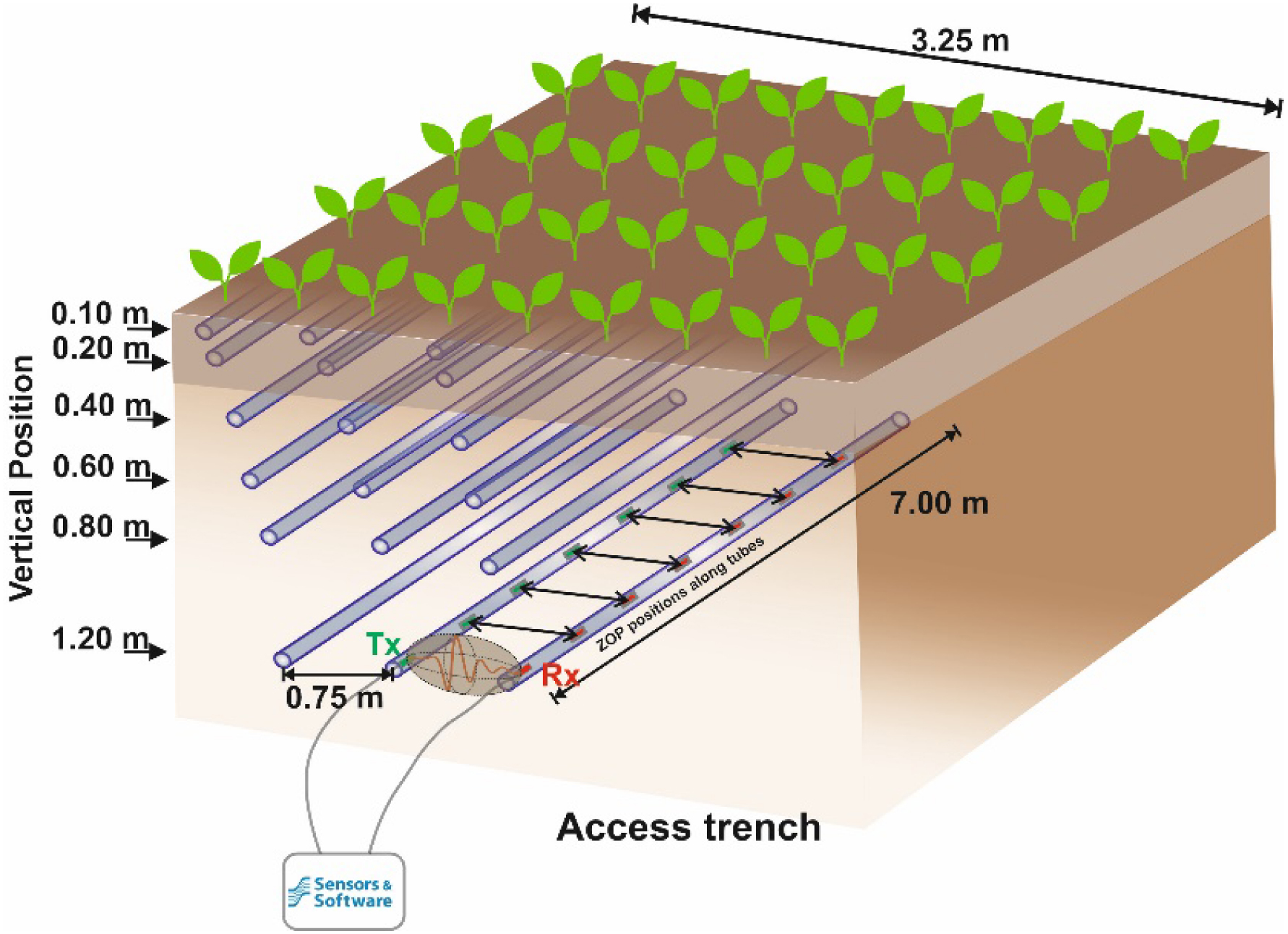
2.2. Root volume fraction based on trench wall counts
To use realistic field root information with sufficient spatial resolution, we used root count density (RCD) values obtained on trench walls of the field MR field facilities in Selhausen for maize (cultivar Zoey) (ibid.). In 2017, trenches were dug next to the field MR facilities to count RCD in an installed 3.75 cm × 3.75 cm grid, see Figure 2a–c (Klotzsche, Lärm, et al., 2019; Morandage et al., 2021). Using the RCD (Figure 2d), the RVF was calculated for each grid cell. First, we derived the root length (RL) per grid cell dimensions
| \begin {equation}\label {eq1} \mathrm {RL}=(\mathrm {RCD}\cdot A_{\mathit {grid}})\cdot L_{\mathit {grid}}, \end {equation} | (1) |
| \begin {equation}\label {eq2} \mathrm {RV}=\mathrm {RL} \cdot \uppi \cdot \frac {d_{\mathit {max}}^{2}}{4} , \end {equation} | (2) |
| \begin {equation}\label {eq3} V_{\mathit {soil}}= A_{\mathit {grid}} \cdot d_{\mathit {max}} \end {equation} | (3) |
| \begin {equation}\label {eq4} \mathrm {RVF}= \frac {\mathrm {RV}}{V_{\mathit {soil}}} \end {equation} | (4) |
Overview of the trench wall counts to derive the root count density. (a) Finalized trench perpendicular to the maize crop rows. (b) Grid on the trench wall, in which the roots were counted. (c) Schematic illustration of the trench wall root counts for one grid cell with a size of 3.75 cm and (d) Results for the root count density for RUT, adapted from (Klotzsche, Lärm, et al., 2019).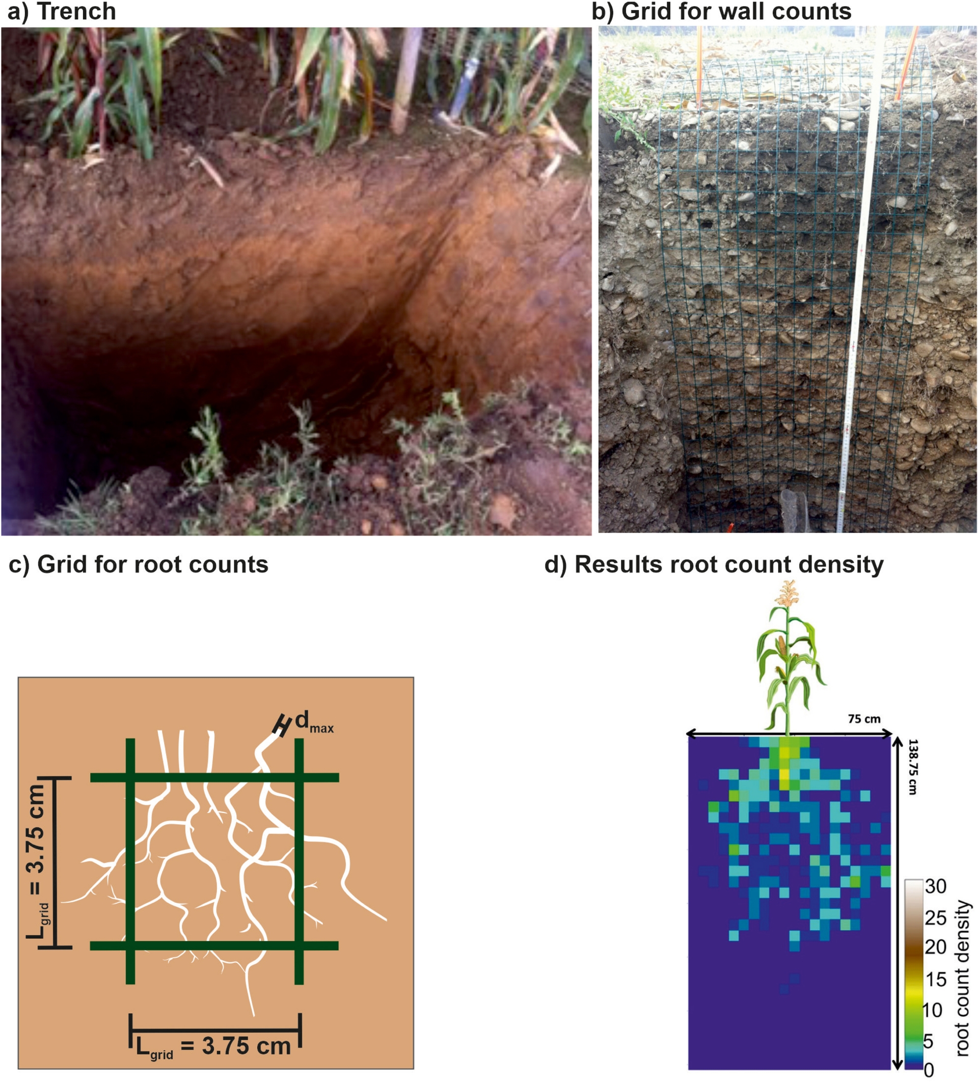
For the crop growing season 2017, we noticed that the distribution of RVF varied for the different soil types of field MR facilities (Figure 3). For RUT the highest number of roots was present close to the surface and decreased with increasing depth (Figure 3a,c). Additionally, the RVF distribution in the horizontal axis was less distributed than for RLT. For RLT the RVF indicated higher amounts of roots in general but also indicated a more complex distribution in both directions of the recorded profile (Figure 3b,d). The mean RVF per depth (Figure 3c,d), which showed a similar depth distribution of RVF as shown in Morandage et al. (2021). For RUT a mean value of ∼3% and maximum value of ∼13% for the shallow depths was observed, which decreased with increasing depth. For RLT the mean RVF was higher by up to 10% at a depth of 0.6 m and reached an overall maximum of 20% at 0.2 m depth and between 0.6 m and 0.8 m depth.
RVF for both field MR facilities with (a,b) RVF values calculated for every grid cell and then interpolated to a cell size of 1 cm. (c,d) RVF depths profiles for RUT and RLT with corresponding mean, standard deviation, maximum and minimum distribution.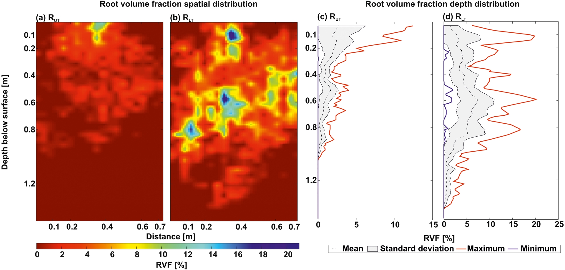
2.3. Soil water content derived from crosshole GPR data considering roots
For the synthetic GPR data, the 𝜀r of the medium was obtained by picking the first arrival time of the GPR EM waves. For more processing details (especially for field measurements), we refer to Klotzsche, Lärm, et al. (2019). Utilizing the picked travel times and considering low-loss and non-magnetic soils (Jol, 2009), the EM velocity v (distance between Tx and Rx is 0.75 m) could be transformed into the 𝜀r of the bulk material with
| \begin {equation}\label {eq5} \varepsilon _{r}= \sqrt {\frac {c}{v}}, \end {equation} | (5) |
To derive the SWC from the obtained 𝜀r petrophysical or empirical relationship are required (Huisman et al., 2003; Klotzsche, Jonard, et al., 2018). Here the empirical relationship Topp’s equation (Topp et al., 1980) is not used here, since it represents sandy soils and at RUT the soil has a high gravel content was present. A widely used petrophysical volumetric mixing model is the complex refractive index model (CRIM). Mixing models have the advantages that they can consider additional dielectric components next to soil, water and air, such as root fractions. The general form of the mixing model assumes that the soil consists of different phases with different dielectric properties and volume fractions 𝜒. For a system with n dielectric components the general formula is
| \begin {equation}\label {eq7} \varepsilon _{r}^{\alpha }= \sum _{i=1}^n \chi _{i} (\varepsilon _{i})^{\alpha }, \end {equation} | (6) |
Illustration of the soil system for the soil-plant continuum: (a) three-phase and (b) four-phase soil system including roots.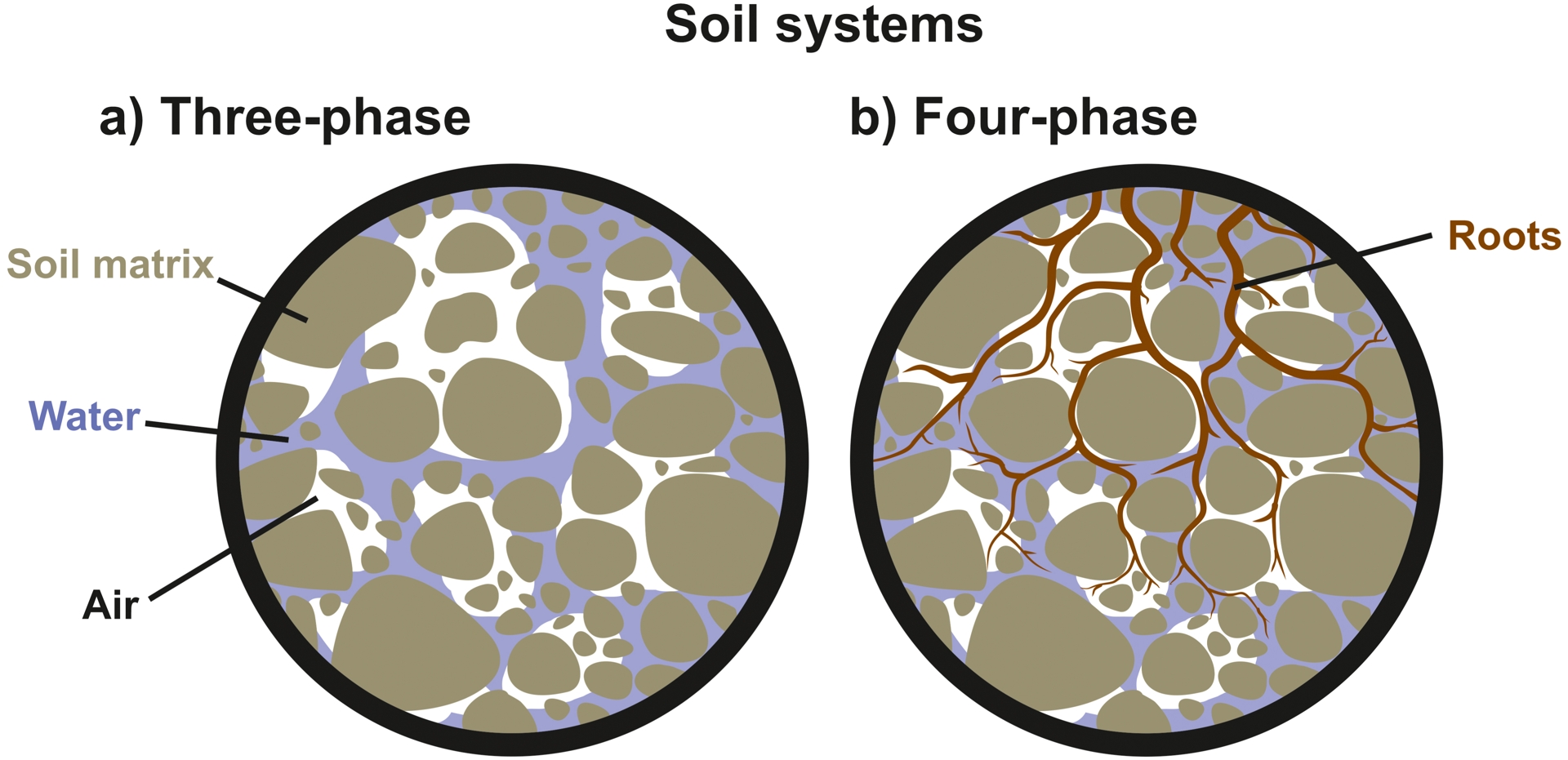
Using these values, we can transform Equation (6) to calculate the bulk permittivity 𝜀r of a three-phase soil system
| \begin {equation}\label {eq8} \varepsilon _{r} = ((1-\phi )\cdot \sqrt {\varepsilon _{s}} + \mathrm {SWC}\cdot \sqrt {\varepsilon _{w}} + (\phi -\mathrm {SWC}))^{2}, \end {equation} | (7) |
| \begin {equation}\label {eq9} \mathrm {SWC}= \frac {\sqrt {\varepsilon _{r}} -( 1-\phi ) \sqrt {\varepsilon _{s}} -\phi } {\sqrt {\varepsilon _{w}} -1} . \end {equation} | (8) |
Note that, when a three-phase system is applied to derive the SWC, this SWC cannot distinguish between water present in the soil or water present in the roots. Especially for row crops, such as maize, with spatially varying roots distribution in the field, the uncertainty on the SWC without considering roots information can be high and the SWC can therefore be over estimated. Therefore, to improve the SWC estimation, which is available to the crops, we need to extend the three-phase soil system by a fourth phase, which considers the root volume inside the pore space (Figure 4b). Thereby, we assume that the porosity equals the summations of RVF, water in the pores and air. Extending Equation (7) with the RVF and the corresponding permittivity of the roots 𝜀R, we derive:
| \begin {eqnarray} \varepsilon _{r} &=& \left ( ( 1-\phi )\cdot \sqrt {\varepsilon _{s}} + \mathrm {SWC}\cdot \sqrt {\varepsilon _{w}} + (\phi -\mathrm {RVF}-\mathrm {SWC}) \right .\nonumber \\ &&\left .+\, \mathrm {RVF}\cdot \sqrt {\varepsilon _{R}}\right )^{2}. \label {eq10} \end {eqnarray} | (9) |
Similar to Equation (8), we can reformulate Equation (9) to derive the SWC for a four-phase soil system
| \begin {equation}\label {eq11} \mathrm {SWC}= \frac {\sqrt {\varepsilon _{r}} - ( 1-\phi )\cdot \sqrt {\varepsilon _{s}} - ( \phi -\mathrm {RVF})- \mathrm {RVF}\cdot \sqrt {\varepsilon _{R}}} {\sqrt {\varepsilon _{w}} -1}. \end {equation} | (10) |
2.4. SWC feasibility study considering roots
To investigate the necessity to account for the RVF, when calculating the SWC, we conducted a feasibility study by calculating the three- and four-phase SWC for a range of 𝜀r, 𝜙 and RVF values. As seen from trench wall counts, the maximum RVF values were about 20% for RLT (see Figure 3b). Therefore, we used a maximum RVF of 20% for this feasibility study. For the calculation of the SWC using Equation (8) and Equation (10), we used 𝜀w = 84 (soil temperature = 10 °C) and 𝜀s = 4 (Klotzsche, Lärm, et al., 2019). There is no quantitative information on the permittivity of the roots and the soil in close promitiy of the roots. Lacking quantitative values we are using a root permittivity 𝜀R of 70, this assumes that crops roots and the soil very close to the roots carry a significant amount of water. Further two different porosities which represent the subsoil porosities were tested, 𝜙 = 0.35 for RLT (Figure 5) and 𝜙 = 0.25 for RUT (see Appendix A).
Results of the feasibility study for (a) three-phase and (b) four-phase CRIM equation for varying 𝜀r and RVF of the soil-plant continuum. Porosity was defined as 𝜙 = 0.35.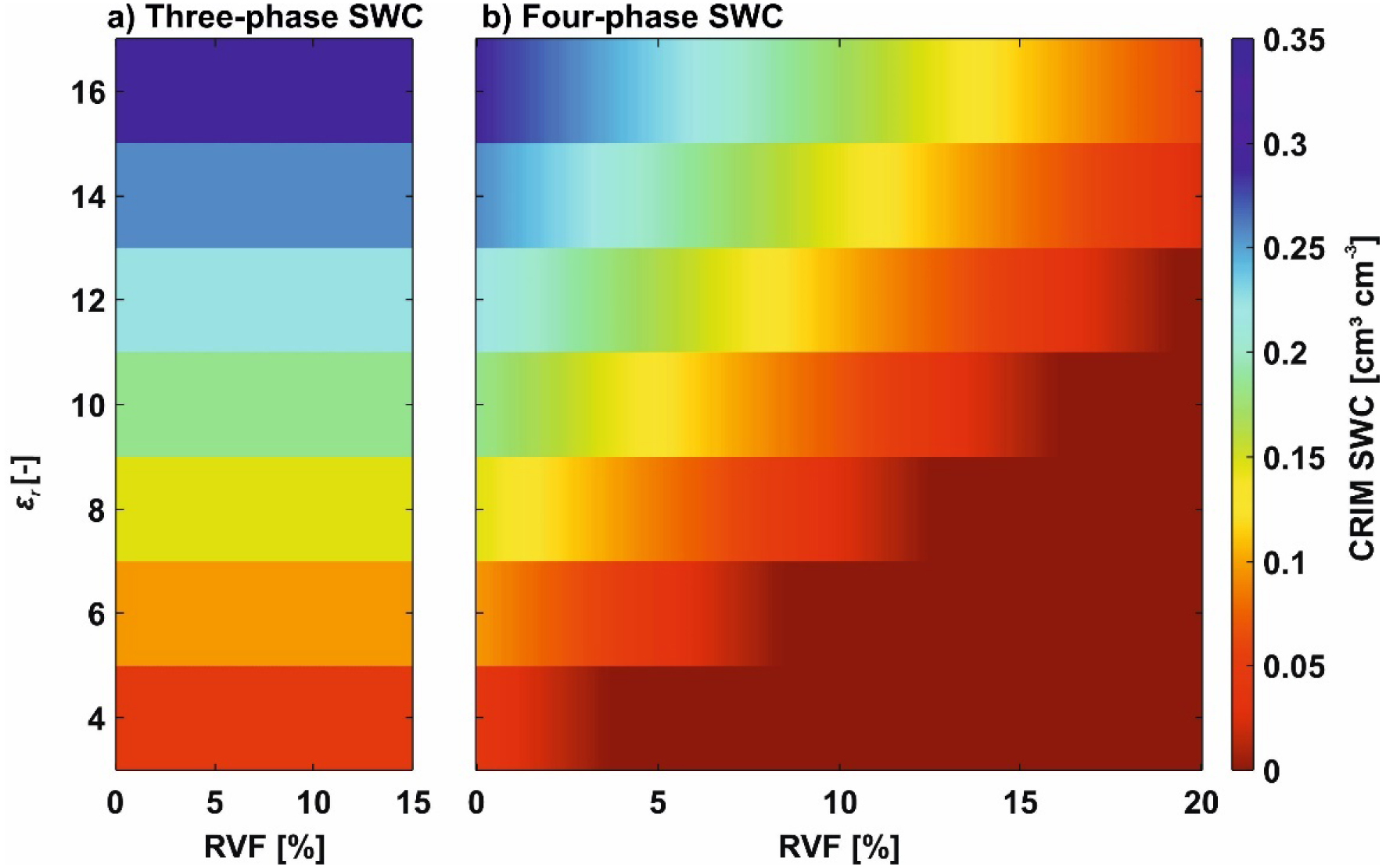
By comparing the results for a range of RVF values for the three-phase and four-phase CRIM, we were able to observe that with increasing root presence, the differences became more considerable (Figure 5). Note that the three-phase SWC was equal to the four-phase SWC with a RVF of 0% (Figure 5a). For lower 𝜀r values the four-phase SWC reached values below zero, in that case in Figure 5b the values were replaced with a SWC of 0 for illustrational purposes.
Analyzing the four-phase SWC depending on the RVF, we noticed a decrease in SWC with an increase in RVF (Figure 5b). Hence, using a three-phase SWC CRIM would lead to SWC overestimation if the root phase is not considered in the calculation. For dry soils (lower permittivity), already a low presence of roots will lead to an absence of water on the soil phase. For example, for a 𝜀r of 4 and a RVF values above ∼3.5%, the four-phase SWC would result in a SWC of 0, while the three-phase SWC would reflect a SWC of ∼0.05. For soils with a 𝜀r of 8, the RVF threshold where the four-phase SWC would reflect a SWC of ∼0 is 12.06%. This effect is even more distinctive for lower porosity soils, see Appendix A. Considering these observations using a three-phase SWC calculation is feasible either if no or very few roots of up to 3% are present or if the root distribution is evenly distributed, e.g., winter wheat. Therefore, for analyzing the variations of SWC related to maize roots, which have in our study a row separation of 0.75 m, a four-phase SWC calculation is recommended, when the RVF exceeds a threshold of 3% in the pore space. Note that for crops with narrow crop row separation, e.g., winter wheat, a more homogeneous root distribution can be assumed, therefore using a three-phase SWC leads to an evenly distributed error.
To further investigate the effect of the root permittivity 𝜀R, on the four-phase SWC, we calculated this using three different 𝜀R, see Figure A2. Two aspects could be observed: First, the four-phase SWC is decreasing, for the same soil permittivity and RVF, when 𝜀R is increasing. Second, with decreasing 𝜀R the four-phase SWC is less affected by the RVF, meaning that for the same soil permittivity the four-phase SWC values do not change as much, when the RVF changes.
2.5. GprMax forward modeling
We performed our synthetic forward modeling study using the open-source electromagnetic simulation software gprMax (Warren et al., 2016). gprMax is a finite difference time domain solver, which can be used to model 2D or 3D electromagnetic waves. As a template for our model domain, we are considering the setup of the field MR facilities cropped with maize. We defined a two-layered model, which includes an above ground air layer (𝜀a = 1) and a soil layer with varying 𝜀r. The model domain has a cell size of 0.01 m and was defined with 1.75 m in x-direction, 2.0 m in the z-directions including 10 cells of perfect matched layers. Like for the field MR facilities, we calculated GPR traces at six different depths with a horizontal spacing of 0.75 m and with Tx and Rx in adjacent rhizotubes. For the simulations a Ricker wavelet was considered as source pulse with a center frequency of 200 MHz similar to the field measurements (Lärm, Bauer, Hermes, et al., 2023). Additional simulations were performed using a center frequency of 500 MHz to investigate whether the various effects can be better discriminated using higher frequency and hence shorter wavelengths.
In this study, we are not investigating the spatial variabilities in the GPR signal along the horizontal axis as we would with the horizontal rhizotubes, rather we are focusing on the comparison of the GPR signal between different set ups of the soil-plant continuum. Therefore, we modeled four different scenarios for the soil-plant continuum where the model consists of: (I) soil, (II) soil and roots, (III) soil and above ground shoot, and (IV) soil, roots, and above ground shoot (Figure 6).
Schematic overview of the different scenarios for RLT with a SWC of 0.2 (cm3⋅cm−3). (a) Scenario I with only soil, (b) Scenario II with soil and roots, (c) Scenario III with soil and shoot and (d) Scenario IV with all the different components soil, roots and above-ground shoot. Note that the permittivity distribution was derived using Equation (9) and 𝜀a = 1.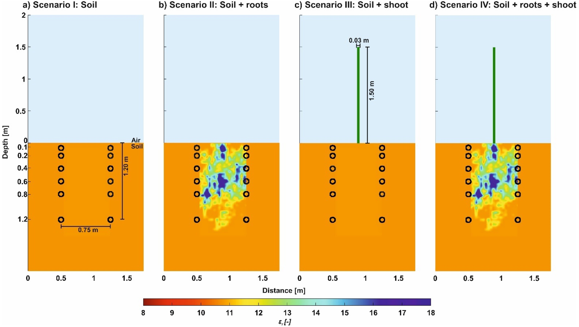
To calculate the 𝜀r, we assumed the below-ground half space to be a three-phase (soil–air–water) system (Equation (7)), when the soil does not include roots (Scenario I and III) and to be a four-phase system (Equation (9)), while the soil includes roots (Scenario II and IV). For Scenario II and IV, we used the RVF fraction distribution (Figure 3a) to calculate the four-phase permittivity for the soil domain, using Equation (9). Since we have modeled only one soil layer, the 𝜀r is constant over the entire soil domain (in the absence of roots). This permittivity is the input for the homogeneous half space (HHS). The two field MR facilities were built in two different soil types, which resulted in different soil 𝜀r, but also in a different root distribution (Figure 3). Previous studies left unanswered whether the effects on GPR traces for shallow depths are caused by above-ground shoots and/or associated precipitation flow processes along the shoots (e.g., Klotzsche, Lärm, et al., 2019; Lärm, Bauer, van der Kruk, et al., 2024). Therefore, we extended the model towards 3D and included a cylindrical object on top of the soil to mimic an aboveground shoot (Scenario III and IV). Note that cylindrical objects cannot be modeled properly in a 2D domain. We assumed the cylinder with a diameter of 0.03 m and a height of 1.5 m similar to extension of maize crops. First, we considered only one maize plant on the soil and second, we extended the model to multiple maize plants (Appendix B, Figure B1). Additionally, we extended the model domain in the z-direction and added shoots with the same dimension as before, with a separation of 0.12 m, which represents the seeding distance of maize. For simplicity, the root distribution was just extended keeping the RVF values constant in y-direction.
Since also the 𝜎 affects the GPR traces, we additional performed simulations where the electrical conductivity of the roots 𝜎R was assumed to be 𝜎R = 0.05 (S⋅m−1) (Rao et al., 2019) in contrast to the 𝜎 of the soil of 0.015 S/m. 𝜎R is usually not constant for the entire root system, it may vary with root age, root order and root diameter, see Rao et al. (ibid.). Furthermore, they investigated in their simulation study, that the electrical conductivity of the roots may change with the root growth away from the root collar and found conductivities between 𝜎R = 0.0154–0.03 (S⋅m−1) for roots up to three weeks old. Since the root system used in this study was mature, nevertheless to account for different conductivities, we used an additional root electrical conductivity of 𝜎R = 0.03 (S⋅m−1).
Under consideration of the different simulation configurations, we calculated GPR traces for a range of realistic expected permittivity values for dry and saturated conditions for both facilities (Table 1).
Overview of the gprMax input parameters for the two field MR facilities and the different SWC conditions.
| RUT | RLT | ||||||
|---|---|---|---|---|---|---|---|
| 𝜙 | (−) | 0.25a | 0.35a | ||||
| 𝜀w | (−) | 84a,b | |||||
| 𝜀s | (−) | 4.7a | 4.0a | ||||
| Input SWC | (cm3⋅cm−3) | 0.05 | 0.15 | 0.25 | 0.10 | 0.20 | 0.35 |
| Input 𝜀r | (−) | 5.22 | 9.62 | 15.35 | 6.08 | 10.78 | 20.32 |
| 𝜎s | (S⋅m−1) | 0.015 | |||||
| 𝜎R | (S⋅m−1) | 0.03/0.05d | |||||
| GPR frequency | (MHz) | 200/500 | |||||
3. GPRMAX simulations
3.1. Model scenarios and SWC conditions
Considering the four introduced scenarios (Figure 6), GPR signals were modeled using a 200 MHz source wavelet for various soil properties (𝜙,𝜀s) and different SWC conditions. Additionally for Scenario III and IV we modeled multiple maize crops (results shown in Appendix B).
In the first step, we assumed for the four scenarios intermediate SWC conditions for both field MR facilities using a SWC of 0.15 and 0.20 for RUT (Figure 7a) and RLT (Figure 7b), respectively. The differences between the two facilities and their related traces are mainly caused by increased SWC for RLT and hence increased travel time of the EM waves and the different RVF distributions. As for depths below 0.6 m, a reflected wave from the air–soil interface can be observed after 20 ns. We observed generally similar phase and amplitudes with shifts in arrival times between the two facilities. The effects of the varying root distribution in the soil influenced the GPR signals for the different depths could be seen when comparing Scenario I and II. We first noticed a difference in the travel times, whereas the first arrival of the EM wave was delayed for Scenario II (Figure 7). This effect differed between the field MR facilities, whereas with higher SWC of RLT caused the travel time difference between Scenario I and II to increase and the travel time differences for RLT were larger than for RUT. This time shift was caused by the increased 𝜀r associated with the RVF and therefore an overall decreased wave velocity and hence resulted in later arrival times.
GPR traces modeled for the four scenarios for 200 MHz, where the black, blue, red and green solid line indicate Scenario I, II, III and IV for the different depths of the field MR facilities, respectively. The corresponding traces are shown for the different field MR facilities for (a) RUT with a SWC of 0.15 (cm3⋅cm−3) and (b) RLT with a SWC of 0.2 (cm3⋅cm−3).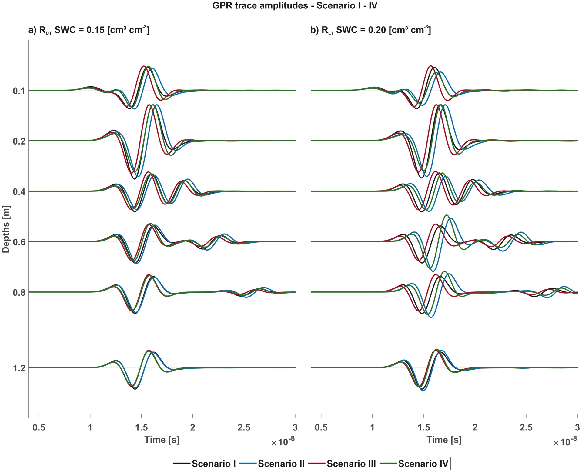
Under consideration of the presence of the above-ground shoot Scenarios III and IV, we noticed the same influence of roots, where the first arrival was delayed, and the amplitudes were smaller (Figure 7). But in the uppermost depths 0.1 m to 0.4 m, we could see later EM wave arrivals, which were not present without the above-ground shoot. Upon considering not just one, but multiple above-ground shoots, we were able identify multiple reflections in the uppermost depths (Appendix B). Generally, we noticed the highest impact on the GPR traces and their travel times in the presence of the root systems rather than the above-ground shoot.
Using the modeled GPR traces, the corresponding 𝜀r were derived using the first arrival times. By comparing the input 𝜀r of the soil with the modeled 𝜀r, we clearly notice that with increasing depth and permittivity the error decreased (Table 2). In general, the modeled permittivities underestimated the input permittivity. The largest errors were observed for the depth 0.1 m, where the error showed values between −51.22% and −56.51% for RUT (SWC = 0.15 cm3⋅cm−3) and RLT (SWC = 0.20 cm3⋅cm−3). This was related to the fact that the direct ground wave and the critical refracted air wave were interfering with the shallowest depth of 0.1 m depth (Klotzsche, van der Kruk, et al., 2016). These wave interactions were present in all scenarios and no clear differentiation between the two events was possible. Note, these wave interactions are more significant for dry conditions rather saturated soils. Therefore, when using the standard analysis tool of picking the first arrival time, this data should be excluded interpretation, since interferences caused an underestimation of the permittivity (Figure 7, Table 2). Consequently, this depth was excluded from the detailed analysis. Note, only full-waveform inversion (FWI) approaches which consider a full three-dimensional electromagnetic wave propagation model would allow to retrieve soil properties from those shallow data (ibid.). Given the impact of sensing volume (SV) of a 200 MHz GPR system on low-permittivity soils, operating at a higher frequency could be an improvement, as it would decrease the SV. For depth 0.2 m this error was already significantly lower, between −9.68% and −15.54%, for the remaining depths the errors were smaller than 1% (without considering roots). While using a similar acquisition setup and GPR measurement frequencies one needs to take extra care to results in the shallow depths, especially for dry soil conditions or less conductive soils.
Modeled 𝜀r results for Scenario I–IV for RUT and RLT and SWC = 0.15 and 0.20 (cm3⋅cm−3), respectively. The error between the input 𝜀r and the modeled 𝜀r is provided in brackets below. Note that Scenario I and II were modeled in 2D, while Scenario III and IV were modeled in 3D.
| RUT | RLT | ||||||||
|---|---|---|---|---|---|---|---|---|---|
| Scenario | Scenario | ||||||||
| I | II | III | IV | I | II | III | IV | ||
| SWC | 0.15 (cm3⋅cm−3) | 0.20 (cm3⋅cm−3) | |||||||
| 𝜀r in soil | 9.62 (−) | 10.78 (−) | |||||||
| Modeled 𝜀r | 0.1 | 4.39 (−54.34%) | 4.40 (−54.22%) | 4.69 (−51.22%) | 4.71 (−51.06%) | 4.69 (−56.51%) | 4.70 (−56.40%) | 5.00 (−53.66%) | 5.01 (−53.50%) |
| 0.2 | 8.15 (−15.28%) | 8.30 (−13.71%) | 8.46 (−12.03%) | 8.68 (−9.68%) | 8.89 (−17.48%) | 9.10 (−15.54%) | 9.24 (−14.30%) | 9.52 (−11.68%) | |
| 0.4 | 9.62 (0.02%) | 10.05 (4.57%) | 9.62 (0.0%) | 10.03 (4.26%) | 10.77 (−0.06%) | 12.70 (17.85%) | 10.7 (0.32%) | 12.6 (17.25%) | |
| 0.6 | 9.62 (0.02%) | 10.02 (4.19%) | 9.62 (0.0%) | 10.00 (4.00%) | 10.77 (−0.06%) | 13.75 (27.58%) | 10.74 (0.32%) | 13.67 (26.83%) | |
| 0.8 | 9.62 (0.02%) | 9.78 (1.66%) | 9.62 (0.0%) | 9.76 (1.49%) | 10.77 (−0.06%) | 13.07 (21.30%) | 10.74 (0.32%) | 12.9 (20.32%) | |
| 1.2 | 9.62 (0.02%) | 9.61 (−0.04%) | 9.62 (0.0%) | 9.59 (−0.25%) | 10.77 (−0.06%) | 11.10 (2.95%) | 10.74 (0.32%) | 11.00 (2.04%) | |
When we compared the errors of Scenario I and III, to estimate the influence of the above-ground shoot on the GPR traces, the error decreased between the input and modeled permittivity, e.g., for depth 0.2 m at RUT (SWC = 0.15 cm3⋅cm−3) the error for Scenario I was −15.28% and for Scenario III −12.03% (Table 2). This effect was even more present under consideration of multiple above-ground shoots, here for Scenario III an error of −9.92% was present (Appendix B, Table B1). Since we only considered the first arrival of the traces to derive the modeled permittivity the errors for the scenarios without the above-ground shoot and the one with shoot were not significant. Note that, the shoots seemed to only affect later arriving reflections in the signal and therefore the first arrival time picking was only slightly affected.
In a second step, we compared the effect of the different SWC scenarios for both facilities on the GPR traces. Since we noticed that the above-ground shoot had only minor effects, we concentrated here on Scenario I and II in 2D. We modeled GPR traces for a set of SWC values, which were common for both field MR facilities (low, intermediate, and high SWC conditions, see Table 1). Generally, the traces for both scenarios were quite similar, while differences became more evident with increasing SWC (Figure 8a–c and d–f). The difference in the GPR traces varied between the different SWC conditions and the field MR facilities (different root distributions). Considering the entire phase of the traces, we noticed differences in for the first cycle amplitude and in the maximum amplitude, e.g., RUT depth 0.2 m and RLT depth 0.2 m 0.6 m (Figure 8a,d—grey circles). With increasing SWC the travel time difference between Scenario I and II increased and the travel time differences for RLT were larger than for RUT. The travel time shift was caused by the increased permittivity associated with the RVF and therefore an overall decreased wave velocity resulted in later arrival times. Additionally, for some depths a phase shift in late arrivals present. Especially recognizable for RLT at depths 0.6 m and 0.8 m, again associated with the highest RVF area (Figure 8b,e—black ellipse).
GPR traces modeled for various SWC, where the black and blue solid line indicates Scenario I and II for the different depths of the field MR facilities. The corresponding traces are shown for the different field MR facilities and different soil water content conditions (a–c) for RUT and (d–f) for RLT. The grey circles indicate the first cycle amplitude differences between, the red lines indicate the travel time difference, and the black ellipse indicates the phase shift for the later EM wave arrivals, between Scenario I and II, respectively.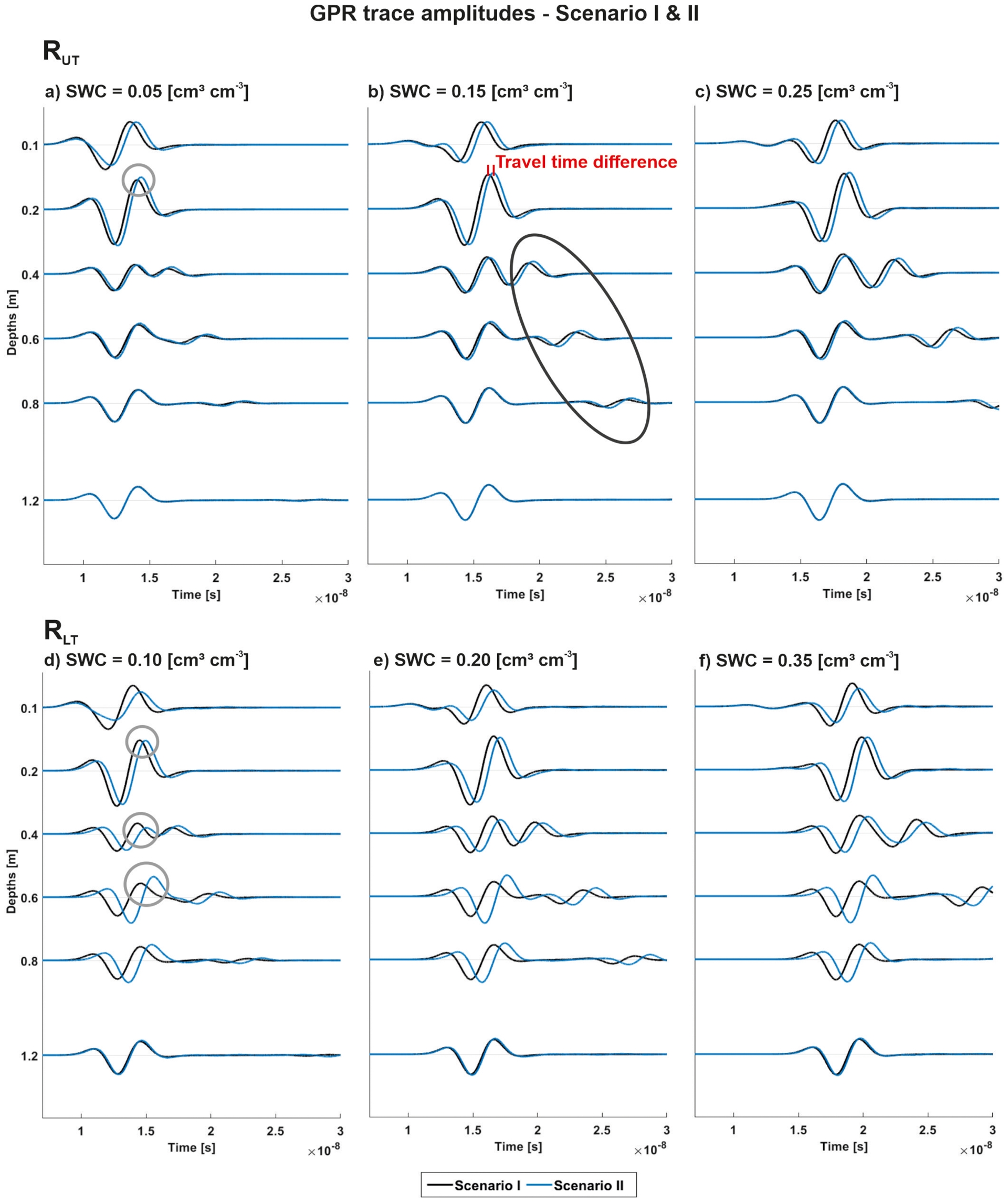
To quantify these phase shifts, we estimated the travel times differences of the maximum amplitude (e.g., Figure 8b—red lines, Table 3). For RUT the largest time difference was observed for 0.2 m depth and for RLT for 0.6 m depth, which exchange with is linked to the high RVF values. Additionally, we noticed an increased difference with increasing SWC. The influence of the RVF on the amplitude of the traces is especially recognizable for RLT (Figure 8d–f, Table 3).
Travel time differences of the maximum amplitude between Scenario I and II, for RUT and RLT.
| Travel time differences | |||||||
|---|---|---|---|---|---|---|---|
| RUT | RLT | ||||||
| SWC | (cm3⋅cm−3) | 0.05 | 0.15 | 0.25 | 0.1 | 0.2 | 0.35 |
| Depth | (ns) | ||||||
| 0.2 | (m) | 0.31 | 0.37 | 0.40 | 0.46 | 0.50 | 0.46 |
| 0.4 | 0.20 | 0.24 | 0.22 | 0.71 | 0.64 | 0.66 | |
| 0.6 | 0.13 | 0.16 | 0.17 | 1.00 | 1.02 | 1.06 | |
| 0.8 | 0.07 | 0.06 | 0.07 | 0.87 | 0.85 | 0.88 | |
| 1.2 | 0.01 | 0.01 | 0.00 | 0.09 | 0.10 | 0.11 | |
For all the SWC conditions and both field MR facilities the modeled 𝜀r was lower than the input 𝜀r, see Table 4. The highest error between these permittivities was present in the uppermost depths originated from by wave interferences caused by the air layer, which agreed with the findings from Figure 8a–f. Note, these wave interferences were also partly present at a depth of 0.2 m, especially for particularly dry soil conditions with low permittivities. Starting from a depth of 0.4 m, the different wave types began to be separately noticeable, and the direct wave was less affected by the reflection from the subsurface, which arrived later in time (Figure 8b,e, black circle). For increased 𝜀r/SWC these reflections became clearer and more distinct. Note that both field MR facilities were affected by these wave interferences, although RLT was less impaired since the overall 𝜀r is higher than for RUT.
𝜀r results for Scenario I and II for RUT and RLT, for different SWC conditions. The error between the input 𝜀r and the modeled 𝜀r is provided in brackets.
| RUT | RLT | |||
|---|---|---|---|---|
| Scenario I | Scenario II | Scenario I | Scenario II | |
| SWC | 0.05 | 0.10 | ||
| 𝜀r in soil | 5.22 | 6.08 | ||
| 0.1 | 3.06 (−41.3%) | 3.10 (40.67%) | 3.36 (−44.71%) | 3.39 (−44.26%) |
| 0.2 | 4.83 (−7.49%) | 5.15 (1.36%) | 5.55 (−8.81%) | 5.98 (−1.68%) |
| 0.4 | 5.21 (0.13%) | 5.54 (6.23%) | 6.09 (0.08%) | 7.55 (24.08%) |
| 0.6 | 5.21 (0.13%) | 5.50 (5.39%) | 6.09 (0.08%) | 8.29 (36.19%) |
| 0.8 | 5.21 (0.13%) | 5.33 (2.18%) | 6.09 (0.08%) | 7.79 (28.02%) |
| 1.2 | 5.21 (0.13%) | 5.22 (−0.06%) | 6.09 (0.08%) | 6.33 (4.01%) |
| SWC | 0.15 | 0.20 | ||
| 𝜀r in soil | 9.62 | 10.78 | ||
| 0.1 | 4.39 (−54.34%) | 4.40 (−54.22%) | 4.69 (−56.51%) | 4.70 (−56.40%) |
| 0.2 | 8.15 (−15.28%) | 8.30 (−13.71%) | 8.89 (−17.48%) | 9.10 (−15.54%) |
| 0.4 | 9.62 (0.02%) | 10.05 (4.57%) | 10.77 (−0.06%) | 12.70 (17.85%) |
| 0.6 | 9.62 (0.02%) | 10.02 (4.19%) | 10.77 (−0.06%) | 13.75 (27.58%) |
| 0.8 | 9.62 (0.02%) | 9.78 (1.66%) | 10.77 (−0.06%) | 13.07 (21.30%) |
| 1.2 | 9.62 (0.02%) | 9.61 (−0.04%) | 10.77 (−0.06%) | 11.10 (2.95%) |
| SWC | 0.25 | 0.35 | ||
| 𝜀r in soil | 15.35 | 20.32 | ||
| 0.1 | 5.77 (−62.39%) | 5.78 (−62.33%) | 6.82 (−66.43%) | 6.83 (−66.41%) |
| 0.2 | 11.62 (−24.25%) | 11.69 (−23.83%) | 14.31 (−29.58%) | 14.43 (−28.99%) |
| 0.4 | 15.35 (0.01%) | 15.90 (3.60%) | 20.32 (0.00%) | 22.96 (12.98%) |
| 0.6 | 15.35 (0.01%) | 15.87 (3.41%) | 20.32 (0.00%) | 24.50 (20.57%) |
| 0.8 | 15.35 (0.01%) | 15.55 (1.36%) | 20.32 (0.00%) | 23.51 (15.71%) |
| 1.2 | 15.35 (0.01%) | 15.35 (0.01%) | 20.32 (0.00%) | 20.78 (2.26%) |
For Scenario II at RUT we noticed, that only for the depth 1.2 m for all SWC conditions, the error between the input 𝜀r and the modeled 𝜀r was less than 1% (Table 4, Figure 9) indicating that the roots had a significant effect on the 𝜀r values and in most cases lead to an increased 𝜀r. Interestingly to notice, was the effect of the roots for the shallow depth of 0.2 m depth, especially in dry soil conditions, where the errors between the input 𝜀r and the modeled 𝜀r was smaller for Scenario II (Table 4, Figure 9). The additional root phase in soil system reduced the interferences on the first arrival time, which was related to the higher overall 𝜀r in the soil system, where the interferences had less influences. While for Scenario I, the input 𝜀r was identified by the first arrival picking for most cases below 0.4 m depth, for Scenario II the error depended on the presence of roots (Table 4). For example, for RLT the highest errors were observed for the depths 0.6 m and 0.8 m, where also the highest RVF were present (Figure 9).
𝜀r depth distributions for both field MR facilities (a,b), where the input 𝜀r indicated as a solid red line, Scenario I indicated as a dashed black line and Scenario II indicated as a solid blue line.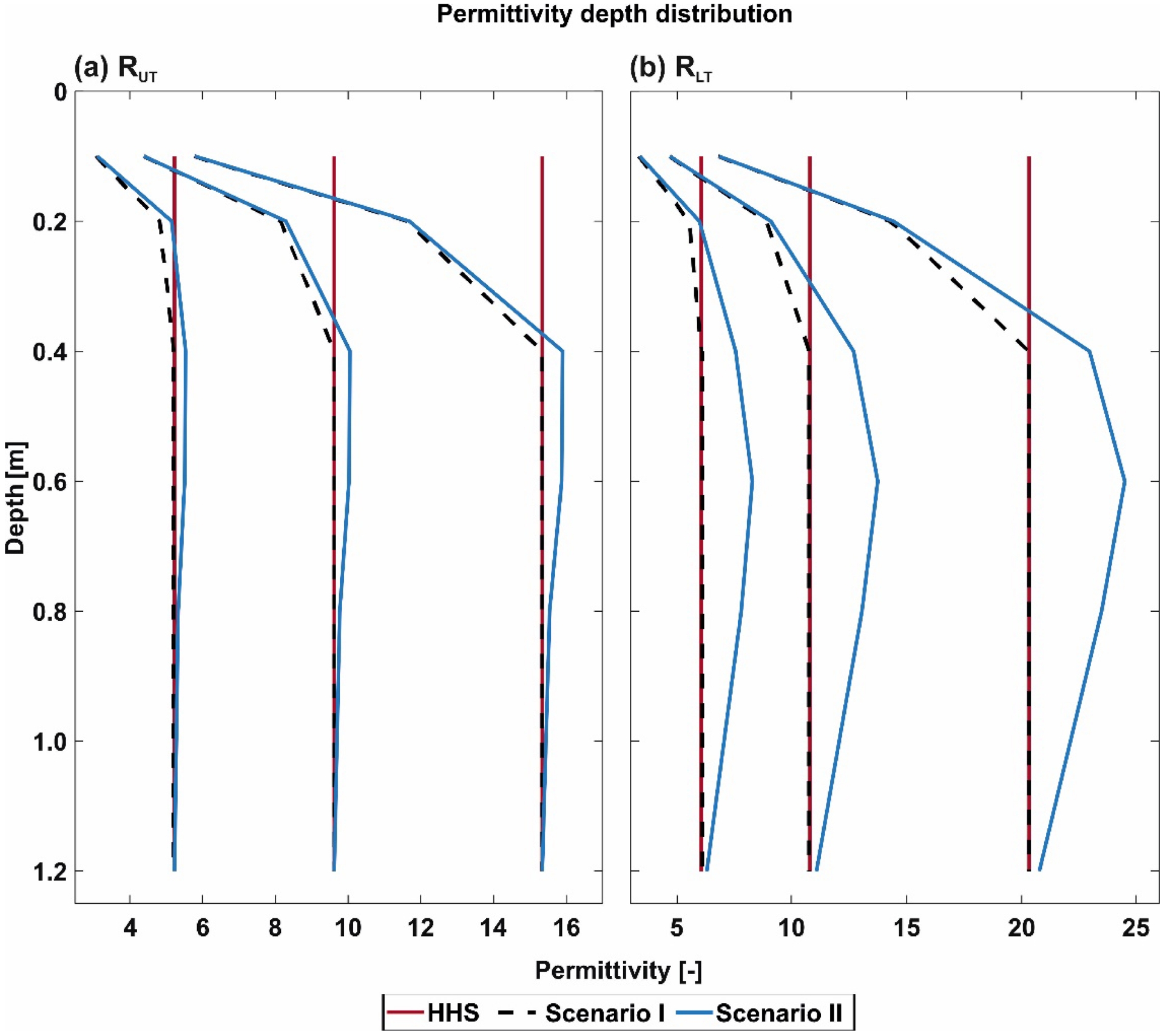
Using the modeled 𝜀r of Scenario I and II, we calculated the three-phase and four-phase SWC (Equations (8) and (10), Figure 10, Table 5). For simplification, we considered the mean RVF per depth rather than the respective SV for each measurement position (see Figure 3c,d). As expected from the feasibility study, if the RVF were not incorporated, the SWC was overestimated. The overall errors were smaller in contrast to higher SWC conditions and decreased with depth. Note that if the RVF was not incorporated in the calculations, errors between −3% to 55% occurred (not considering depth 0.1 m), see Table 5.
SWC depth distributions for both field MR facilities (a,b). The input SWC is indicated as a dashed red line, Scenario I indicated as a solid black line, three-phased SWC for Scenario II indicated as a solid blue line and four-phased SWC for Scenario II indicated as a solid brown line.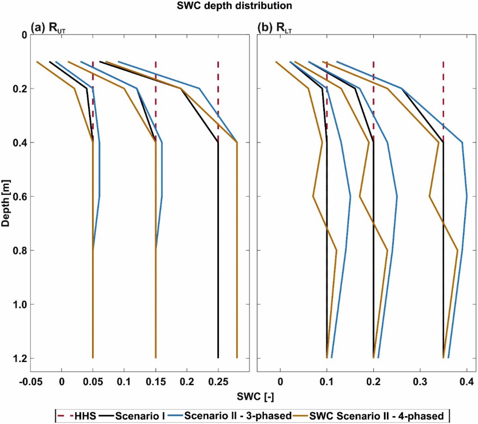
Three-phase SWC for Scenario I, and three-phase and four-phase SWC results for Scenario II for RUT and RLT and different SWC conditions between 0.05–0.35 (cm3⋅cm−3). The error between the three- and four-phase SWC is provided in brackets below.
| RUT | RLT | |||||
|---|---|---|---|---|---|---|
| Scenario I | Scenario II | Scenario I | Scenario II | |||
| SWC | 0.05 (cm3⋅cm−3) | 0.10 (cm3⋅cm−3) | ||||
| SWC (three-phase) | SWC (three-phase) | SWC (four-phase) | SWC (three-phase) | SWC (three-phase) | SWC (four-phase) | |
| 0.1 | −0.02 | −0.01 | −0.04 (157.14%) | 0.02 | 0.02 | −0.01 (−134.78%) |
| 0.2 | 0.04 | 0.05 | 0.02 (−50.00%) | 0.09 | 0.10 | 0.06 (−39.18%) |
| 0.4 | 0.05 | 0.06 | 0.05 (−18.64%) | 0.10 | 0.13 | 0.09 (−36.57%) |
| 0.6 | 0.05 | 0.06 | 0.05 (−17.54%) | 0.10 | 0.15 | 0.07 (−55.33%) |
| 0.8 | 0.05 | 0.05 | 0.05 (0.00%) | 0.10 | 0.14 | 0.12 (−11.43%) |
| 1.2 | 0.05 | 0.05 | 0.050 (0.00%) | 0.10 | 0.11 | 0.10 (−6.60%) |
| SWC | 0.15 (cm3⋅cm−3) | 0.20 (cm3⋅cm−3) | ||||
| 0.1 | 0.03 | 0.03 | 0.01 (−81.48%) | 0.06 | 0.06 | 0.03 (−49.21%) |
| 0.2 | 0.12 | 0.12 | 0.10 (−19.51%) | 0.16 | 0.17 | 0.13 (−22.75%) |
| 0.4 | 0.15 | 0.16 | 0.15 (−6.92%) | 0.20 | 0.23 | 0.19 (−20.94%) |
| 0.6 | 0.15 | 0.16 | 0.15 (−6.33%) | 0.20 | 0.25 | 0.17 (−32.94%) |
| 0.8 | 0.15 | 0.15 | 0.15 (0.00%) | 0.20 | 0.24 | 0.23 (6.64%) |
| 1.2 | 0.15 | 0.15 | 0.15 (0.00%) | 0.20 | 0.21 | 0.20 (−3.40%) |
| SWC | 0.25 (cm3⋅cm−3) | 0.35 (cm3⋅cm−3) | ||||
| 0.1 | 0.06 | 0.09 | 0.07 (−23.91%) | 0.12 | 0.12 | 0.09 (−27.12%) |
| 0.2 | 0.19 | 0.22 | 0.19 (−11.52%) | 0.26 | 0.26 | 0.23 (−14.45%) |
| 0.4 | 0.25 | 0.28 | 0.28 (−3.50%) | 0.35 | 0.39 | 0.34 (−12.99%) |
| 0.6 | 0.25 | 0.28 | 0.28 (−3.50%) | 0.35 | 0.40 | 0.32 (−20.54%) |
| 0.8 | 0.25 | 0.28 | 0.28 (−0.36%) | 0.35 | 0.39 | 0.38 (−4.08%) |
| 1.2 | 0.25 | 0.28 | 0.28 (0.00%) | 0.35 | 0.36 | 0.35 (−1.97%) |
When analyzing the three- and four-phase SWC under consideration of the above-ground shoot (single and multiple), the effects were dominated by the impacts we had already noticed, so that only depth and 0.1 m and 0.2 m indicated different SWC values between single and multiple shoots (Appendix B, Table B2). Concluding that the RVF had the same influence on the error and the difference between the three- and four-phase SWC, as noticed for Scenario I and II, where the error increased with the increased root presence. Note that, changed infiltration patterns, caused funneled precipitation by stem flow, into the soil could not be considered in this study.
In a third step, we characterized the observed wave interferences in more detail. We calculated the corresponding frequency spectra of the GPR traces for Scenario I and II for the intermediate soil conditions of RUT SWC = 0.15 cm3⋅cm−3 and RLT SWC = 0.2 cm3⋅cm−3 (Figure 11). For the frequency spectra for depths 0.2 m and 0.6 m, we observed a center frequency of approximately 200 MHz. The wave interferences at 0.2 m caused a higher amplitude of the frequency spectrum almost twice as high as for depth 1.2 m, see Figure 11a and b. For depth 0.6 m we noticed the interferences of the direct air wave and the refracted wave also in the frequency spectra, causing two peaks in the frequency spectrum, for both field MR facilities, which indicated the partly overlap of the EM waves (Figure 11c,d). Comparing the different scenarios, we observed that for Scenario II the center frequency was slightly reduced caused by the overall increased 𝜀r.
Frequency spectra for a SWC of 0.15 cm3⋅cm−3 and 0.2 cm3⋅cm−3 for RUT and RLT, respectively, for exemplary depths of 0.2, 0.6 and 1.2 m. Frequency spectra for RUT are shown in (a,c) and (e), and for RLT in (b,d) and (f). The black and blue solid line indicates Scenario I and II, respectively.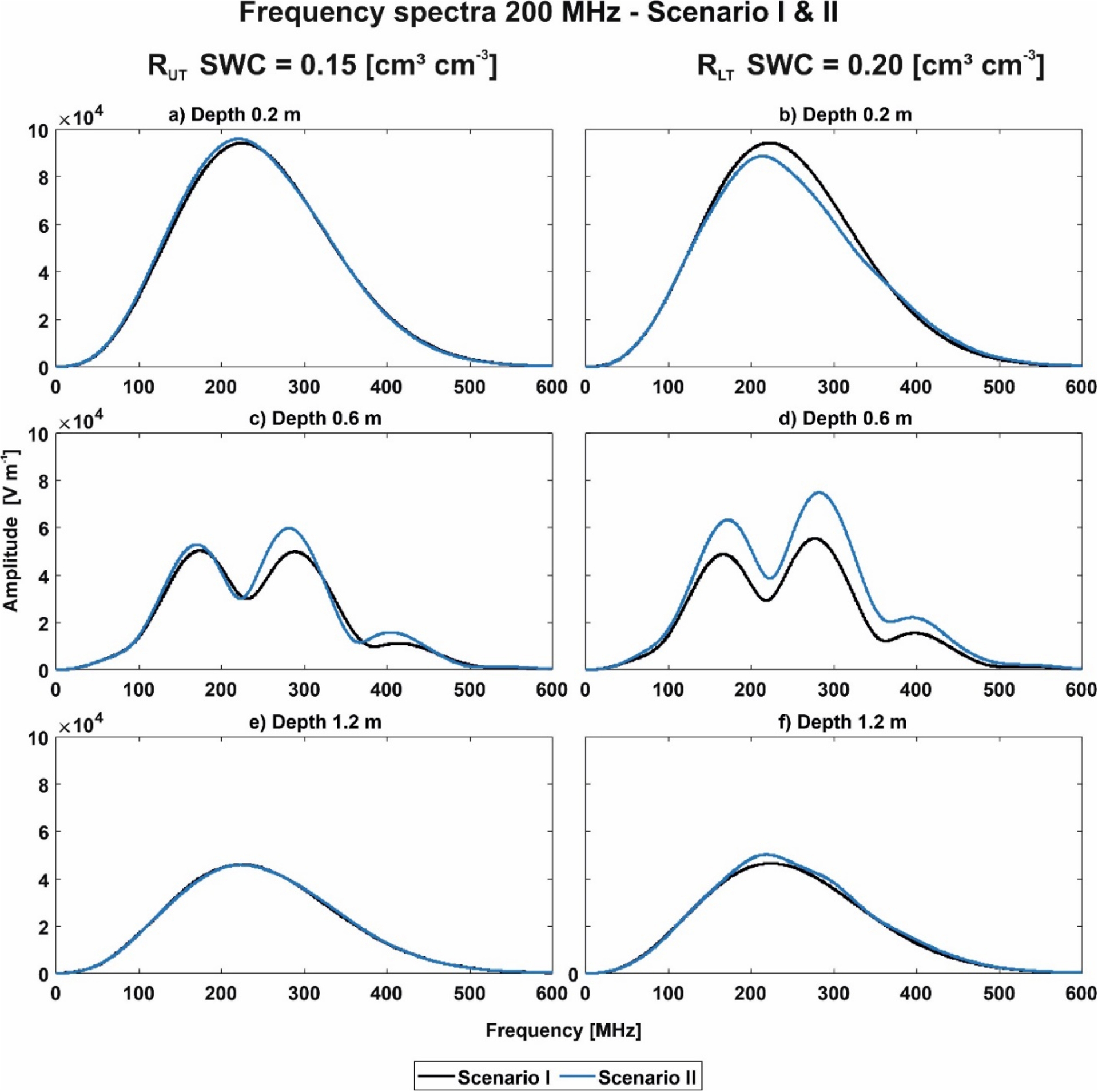
In the frequency spectra of the 200 MHz signal (Appendix B, Figure B2), we observed an influence of the above-ground shoot, but only for the depth of 0.6 m, where the maximum around 300 MHz is significantly larger than for the scenarios without the above-ground shoot. Furthermore, we noticed the same effects on the spectrum as for Scenario I and II, where in the depth 0.2 m an amplitude twice the amplitude as for depth 1.2 m was indicated, caused by the interferences with the reflected and refracted wave. However, no significant difference is noticeable between a single and multiple above-ground shoots.
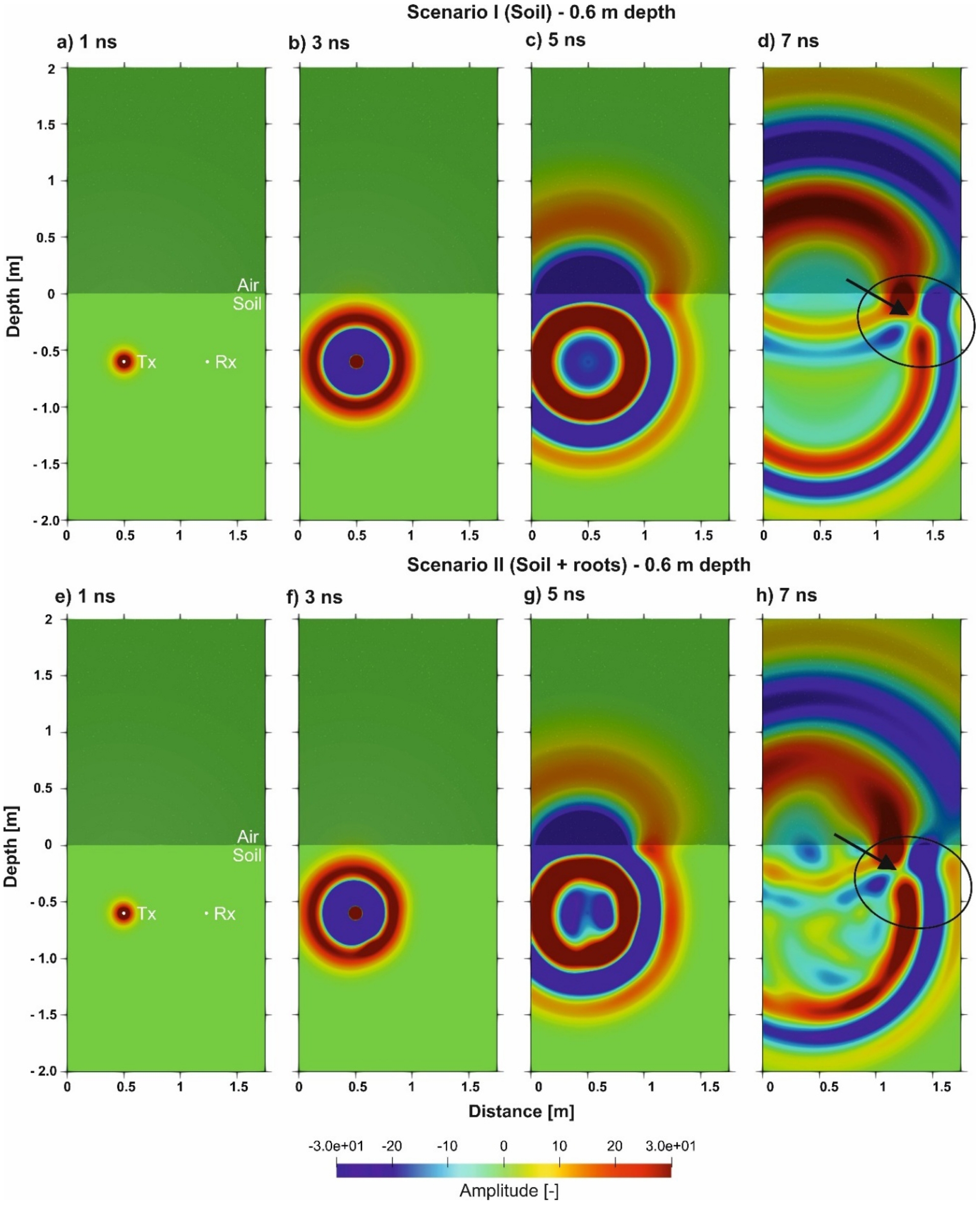
For a better understanding, how the EM waves propagated and interfered in the two-dimensional space with and without root presences, we analyzed image plots for various time steps (1 ns, 3 ns, 5 ns and 7 ns). For both field MR facilities the highest RVF is present at 0.2 m depth, hence we first investigated those EM propagations for RLT with an input SWC of 0.10 cm3⋅cm−3, see Figure 12. Thereby, we noticed for Scenario I, that the EM wave propagated relatively circular and uniform through the soil, whereas for Scenario II, the EM wave showed scatterings and amplitude changes over the model domain. At 3 ns and 5 ns (Figure 12b and c, f and g) the development of the different wave types at the soil–air interface was visible, where the wave in air travels faster than the wave in the soil. At later times of 7 ns (Figure 12d,h) an event was observed with increased amplitude (Figure 12d, black circle). Below, these positive interferences, a time shift and a diminished amplitude were present (Figure 12d, black arrow). Both events were related to the phase and amplitude of the corresponding measured traces (Figure 8). The image plots for the depth 0.6 m for the same scenarios showed overall less wave interferences, although the wave interaction close to the surface was observed as well (see Appendix C, Figure C1).
Image plots (a–d) for Scenario I and (e–h) for Scenario II of the forward modeled electrical field distributions through the model domain for four-time steps when the Tx and Rx are located at 0.2 m depth in the RLT with a SWC of 0.1 (cm3⋅cm−3).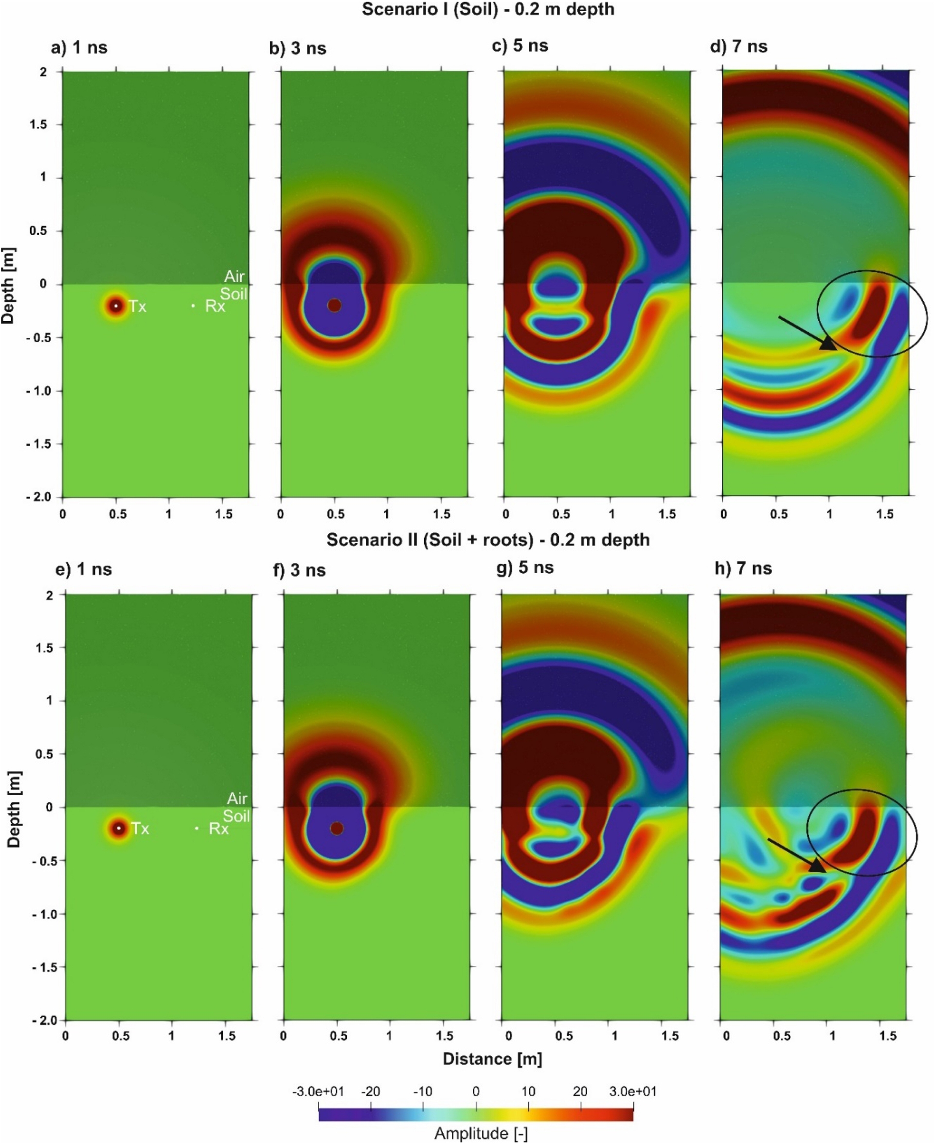
3.2. Root electrical conductivity
We performed simulation with different root electrical conductivities for Scenario I and II with the SWC of 0.15 cm3⋅cm−3 and 0.2 cm3⋅cm−3 for RUT and RLT, respectively (Figure 13). As expected, the models with the increased 𝜎R and hence higher wave attenuation showed a decreased amplitude of the GPR traces. Note that the effect was increased for domains with a higher RVF, e.g., 0.6 m depth. But, overall, only minor differences in the first cycle amplitudes between the traces of the three cases were visible, indicating that the 𝜎R did not have a large effect on the GPR traces. This finding suggests that in further research with more complex soil or/and root models, the different 𝜎R are not a major contributor on the GPR signals rather than the 𝜎S.
GPR traces modeled in 2D for 200 MHz while using different 𝜎R for Scenario II for (a) RUT with an input SWC of 0.15 (cm3⋅cm−3) and (b) RLT with an input SWC of 0.2 (cm3⋅cm−3). The red solid line indicates 𝜎R = 0.015 (S⋅m−1), the blue solid line indicates 𝜎R = 0.05 (S⋅m−1), and the yellow solid line indicates 𝜎R = 0.03 (S⋅m−1). Note that only traces related to the highest RVF region are plotted.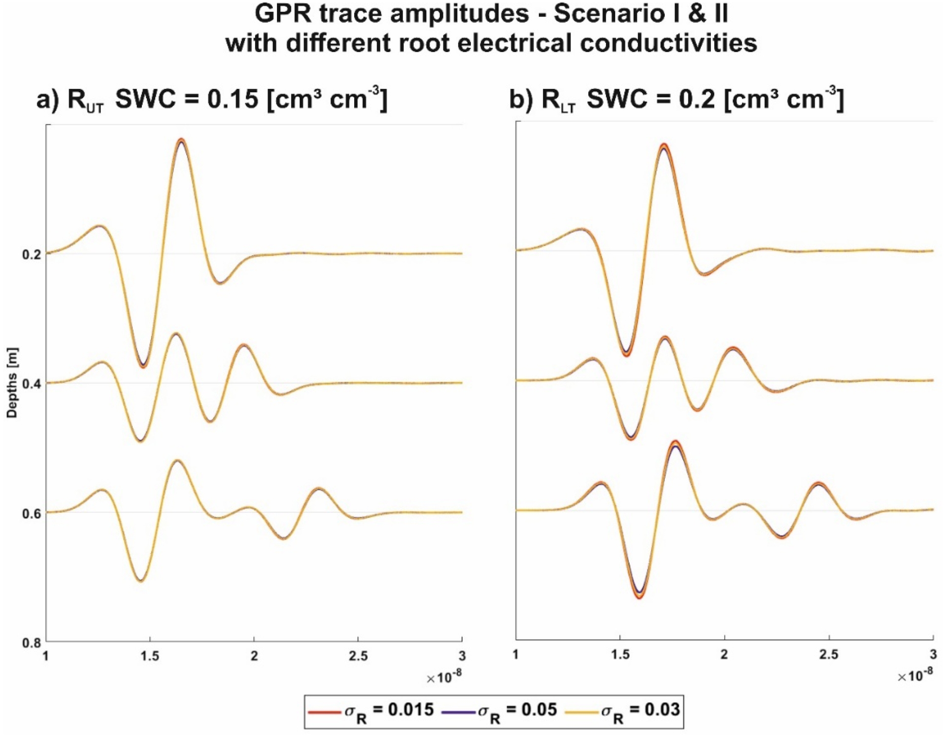
3.3. Measurement frequency
As mentioned previously, a possible improvement in the quantification of permittivity values, particularly at shallow depths, could be achieved by using a higher frequency system. On the one hand, a higher frequency would decrease the SV of the GPR data; on the other hand, the near-field effects could be reduced. Note that, for this setup with a borehole separation of 0.75 m in dry conditions, a 200 MHz system is still partly in the near field of the antennas, causing problems with the first break picking. Therefore, to estimate and possibly enhance the resolution and reconstruction of the medium properties it is necessary to consider the actual SV of the GPR measurement systems. The SV of GPR measurements has the shape of an elongated rotational ellipsoid. The foci of this ellipsoid are the locations of Tx and Rx. The dimensions (size of volume) depend on the distance between Tx and Rx, GPR center frequency, and 𝜀r and hence SWC (Klotzsche, Lärm, et al., 2019). As the recent research related to the field MR facilities focused on 200 MHz data because of commercial availability, the previous simulations were focusing on this measurement frequency. Since roots and the related rhizosphere are in the millimeter to centimeter scale, higher frequency such as 500 MHz would be more suitable. Note that antennae in the GHz range should not be considered since the distance of the rhizotubes, and the wave attenuation and scattering would prevent the detection of the signal. By extending the SV estimation towards 500 MHz, we see that the SV would be reduced by a factor 3 or 4, especially for conditions with higher input 𝜀r/SWC.
We repeated the forward modeling using a Ricker wavelet with a center frequency of 500 MHz to investigate if the interferreing waves and effects caused by the root presence could better be distingished. For an exemplary model scenario, we considered a for RUT und RLT a SWC of 0.15 cm3⋅cm−3 and 0.2 cm3⋅cm−3, respectively (Figure 14a,b). In general, we recognized similar findings as for the 200 MHz simulations: first, we noticed the interference of the direct air wave and refracted air wave, for the 0.1 m depth a small amplitude prior to the first arrival of the EM wave was present. For the 0.2 m depth the interfering wave arrived almost simultaneously with the direct ground wave (Figure 14a,b). For traces at a depth of 0.4 m and 1.2 m, the reflections of the wave at the soil–air-interface were clearly distinguishable (Figure 14a,b, black circles). For the comparison between Scenario I and II, the differences while using a frequency of 500 MHz seemed more significant than using 200 MHz. Overall, we noticed a later first arrival time when including the root phase into the model. While for RUT and the uppermost depths the arrivals times were not significantly different, for the traces below depth 0.8 m for RLT larger offset were observed. Additionally, the interfering waves were affected by this delay in travel time. Interestingly to notice is phase and the amplitude behavior of the traces at depths 0.2 m to 0.6 m for Scenario II for RLT, where the traces showed an increase amplitude for the first direct waves in contrast to Scenario I.
GPR traces modeled in 2D for 500 MHz, where the black solid line indicates Scenario I and the blue solid line represents Scenario II for the different depths of the field MR facilities. The traces are shown for (a) RUT with an input SWC of 0.15 (cm3⋅cm−3) and (b) RLT with an input SWC of 0.2 (cm3⋅cm−3). The dashed black circles indicate the reflections of the wave at the soil–air-interface.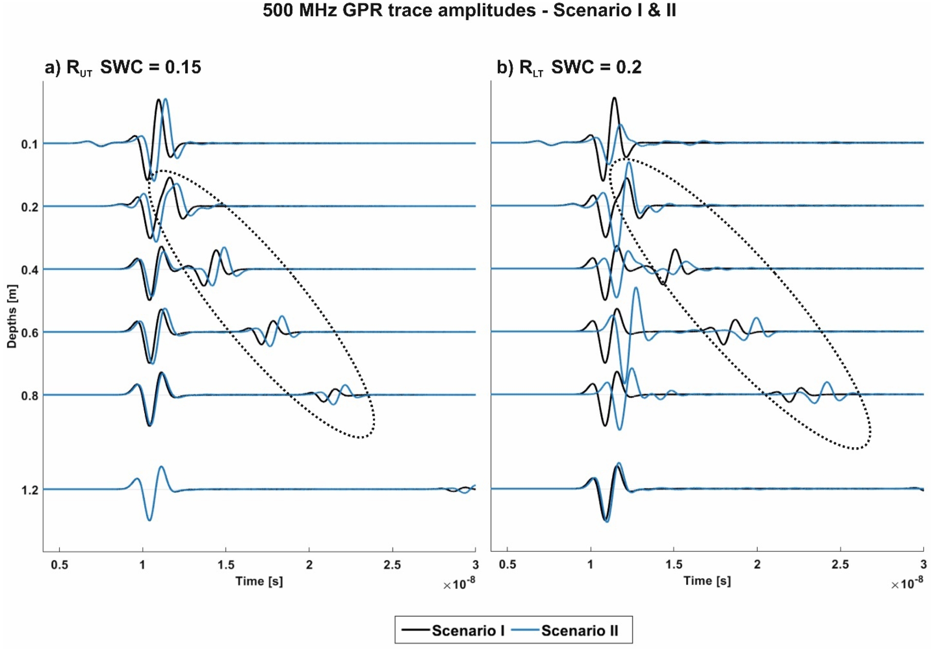
4. Conclusion and outlook
Since currently the effects of roots and the rhizosphere components on the GPR signals are not fully understood we investigated various effects in a numerical study using realistic model scenarios. A feasibility study demonstrated the need that RVF should be considered in the SWC calculations if a threshold of 5% is reached and especially under the consideration of row crops, such as maize. In trench wall root count values above this threshold were observed and therefore we considered this root information as input for our synthetic models. To disentangle the different effects of the soil, water, roots, and above-ground shoots, we considered different scenarios with varying compositions and calculated the corresponding GPR traces. Because we have seen influences by root presence and above-ground shoots on field measurements, we used two field minirhizotron facilities as a template for the setup of the model, with varying soil properties and root distributions.
We observed two major impacts on the GPR signal. First, the air–subsoil interface caused critically refracted air waves and reflections, which were nearly impossible to distinguish from the direct ground wave for shallow investigation depths of 0.1 m (and partly 0.2 m depth). Here, we noticed that an increase in 𝜀r and therefore SWC or root presence (associated with higher 𝜀r), resulted in a better distinction between the different wave types. This effect is caused by the smaller EM wave velocity under higher 𝜀r of the medium the wave is traveling through. Additionally, such effects were minimized when using a higher measurement frequency with shorter wavelength where such events can be better recognized. Note that, also the SV with higher frequencies is reduced and therefore, small-scale variability can better be detected. Second, the presence of roots, which resulted in a 𝜀r increase for the grid cell, lead to an effect on the first arrival time and amplitudes of the GPR trace. This time shift caused an overestimation in SWC, if a conventional three-phase soil system calculation for the soil water content is used. To calculate the soil water content for the soil-plant continuum as a soil system with four phases (soil, air, water, and roots), we used the mean RVF between Tx and Rx. This approach bears the uncertainty of the SV of the GPR measurements, since depending on frequency and bulk 𝜀r of the soil, different SV were present in the shape of an elongated rotational ellipsoid with the foci at the locations of Tx and Rx. When calculating the four-phase SWC all roots present in the ellipsoid should be considered, but the estimation of the number of roots is nearly impossible with the investigation techniques currently available. Here two significant uncertainties arise: First, we are deriving the RVF from a 2D dataset, so therefore we are missing information in the y-dimension. Second, we are using mean 1D RVF for the measurement depths to calculate the four-phase SWC, which does not account for all the roots present in the GPR SV.
Here, modeling approaches, which could provide factors to use either root information derived from root images or trench wall counts, to derive the RVF for a certain soil volume, would be beneficial. Additionally, the estimation of the RVF from the RCD contains uncertainties. We considered the roots to grow straight through the grid and the root diameter to equal over the entire root system. Especially maize roots have a distinct root system architecture with the crown roots (diameter > 2 mm) on top of the soil and close to the shoot. Few studies have investigated the distribution of root diameter distribution in the field, especially considering row crops, such as maize (Buczko et al., 2008). Anderson (1987) found larger maize root diameters within the crop row and Qin et al. (2005) and Schenk and Barber (1980) detected larger root diameters in the topsoil. Furthermore, the used distribution for the RVF is for a mature root system and the trench wall count methods returns quite high values. As Wacker et al. (2024) mentioned the conversion from 2D to 3D root information is challenging. Hence, site-specific decisions are necessary whether a three- or four-phase calcualtion of the SWC should be used.
When considering the root as an individual phase within the soil system, we considered the 𝜀R to be similar to the permittivity of water, but research in the permittivity of roots is rarely available. One of the few studies provided by Attia Al Hagrey (2007) provided a 𝜀R for wood cellulose, depending on the water content between 4.5 < 𝜀R < 22, because of the non-wooden nature of crop roots, realistic values are unknown. We showed that smaller 𝜀R reduce the four-phase SWC and make it more sensitive to changes in RVF, while lower 𝜀R results in higher SWC values that are comparatively less affected by RVF.
Further research could include the investigation of 𝜀R in general but also considering root growth and decay. Incorporating the distribution of the 𝜀R into a root architecture model and combining this with a soil modeling tool for the precise generation of the model domain for the electromagnetic simulation would be more than beneficial to study the influence of the soil components on the GPR signal in more detail. With the here described approach, we adjusted the grid cell 𝜀r under the presence of roots. Since coarse roots, as are present for maize crown roots have diameters >2 mm and are of a wooden texture, they could cause reflection effects in the EM wave. Especially when utilizing high measurement frequencies (500 MHz and above) and surface GPR acquisitions techniques. Additionally, laboratory experiments could be performed under controlled settings to target the retrieval of the root permittivity for different SWC, nutrient, and growth conditions.
One open question raised by the experimental data is how much the above-ground part of the plant influences GPR signals near the surface. To address this, we examined the effects of both single and multiple above-ground shoots. In our static model scenario, where the plant is represented only as a cylinder and infiltration along the stem is ignored, only the late-arrival phases and their amplitudes are affected by the shoots, while the first-arrival times remain unchanged. However, when spatio-temporal processes such as water infiltration along the stem are taken into account, the local dielectric permittivity (𝜀r) beneath the plant can increase, which may delay the first arrivals.
While this study highlights the complex interactions between roots, soil and GPR signals, it also shows the limitations of simplified model scenarios. Although this simulation study is an important first step, further investigations are clearly needed to fully understand the GPR signal, particularly in more realistic and complex soil environments such as those found in row crops and under natural soil conditions. Future research could include additional simulations considering multiple soil layers, among other approaches. Furthermore, with this approach the time component in the soil-plant continuum has not been considered. While infiltration of precipitation and irrigation as well as soil water depletion are taking place, the 𝜀r distribution varies. In this study the SWC conditions and therefore the 𝜀r of the homogenous half space was considered to be constant. The use of a more realistic 𝜀r profile in all dimensions, would be essential here common soil hydraulic modeling tools like HYDRUS-1D could be used to derive 𝜀r profiles (Lärm, Weihermüller, et al., 2025). Further, the influence of soil nutrient/fertilization (Kaufmann et al., 2019), management practices (Blanchy et al., 2020) could be investigated. Further advantages could be provided by using more sophisticated analysis approaches, such as FWI (Klotzsche, van der Kruk, et al., 2016; Klotzsche, Vereecken, et al., 2019; Yu et al., 2022). As observed in this study, effects caused by the root presence, conductivity changes and above-ground shoots are related to later EM wave phases and amplitudes, the FWI approaches have the potential to analyze these effects, but with the downside of increased computational demand and hence additions to data acquisitions should be considered.
Acknowledgments
The manuscript was written through contributions of all authors. This work has partially been funded by the German Research Foundation under Germany’s Excellence Strategy, EXC-2070 - 390732324 - PhenoRob. The authors gratefully acknowledge computing time on the supercomputer JURECA (Jülich Supercomputing Centre, 2021) at Forschungszentrum Jülich under grant no. cjicg41.
Declaration of interests
The authors do not work for, advise, own shares in, or receive funds from any organization that could benefit from this article, and have declared no affiliations other than their research organizations.
Appendix A. Feasibility study for SWC considering roots
When a different porosity (𝜙= 0.25) was present in the soil, the effect that with a certain RVF, the water remaining in the soil was 0, was enhanced for especially dry soil conditions. For a 𝜀r of 4, a RVF values above 2.7% lead to a four-phase SWC of 0, while the three-phase SWC was 0.03. For soil with 𝜀r = 8, the threshold for the RVF, where there was no water left in the soil was RVF = 11.06%.
Results of the feasibility study for (a) three-phase and (b) four-phase CRIM soil water content calculation with varying bulk permittivities and root volume fraction of the soil-plant continuum. Porosity was defined as 𝜙 = 0.25.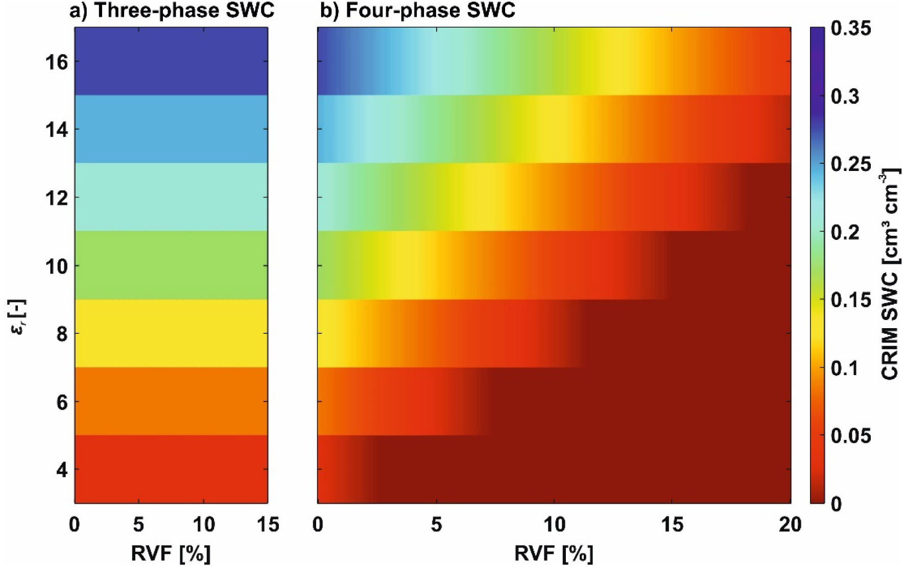
Results of the feasibility study for a four-phase CRIM soil water content calculation with varying bulk permittivities and root volume fraction for different root permittivity values: (a) 𝜀R = 20, (b) 𝜀R = 50, and, (c) 𝜀R = 70.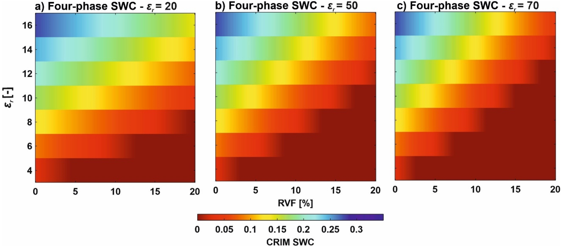
Appendix B. Effects of multiple above-ground shoots
GPR traces modeled for 200 MHz, where the red and green lines indicate Scenario III and IV for the different depths of the field MR facilities, respectively. The solid and dashed line represent the single and multiple above-ground shoots, respectively. The corresponding traces are shown for the different field MR facilities for (a) RUT with a SWC of 0.15 (cm3⋅cm−3) and (b) RLT with a SWC of 0.2 (cm3⋅cm−3).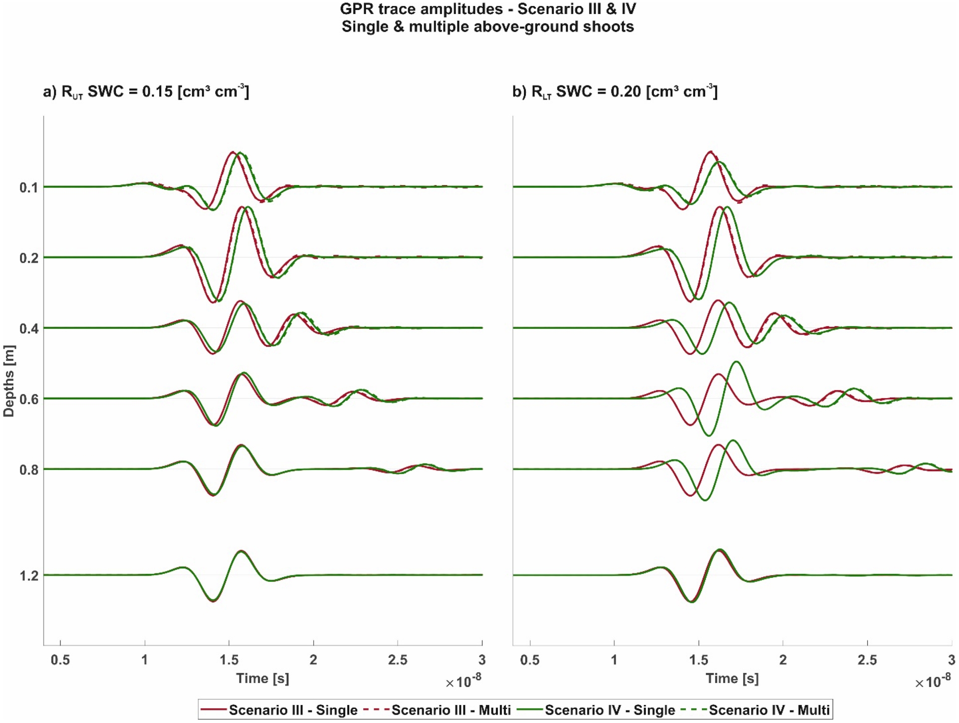
Frequency spectra for a SWC of 0.15 cm3⋅cm−3 and 0.20 cm3⋅cm−3 for RUT and RLT, respectively, for exemplary depths of 0.2, 0.6 and 1.2 m. Frequency spectra for RUT are shown in (a), (c) and (e), and for RLT in (b), (d) and (f). The red and green solid line indicates Scenario III and IV, respectively.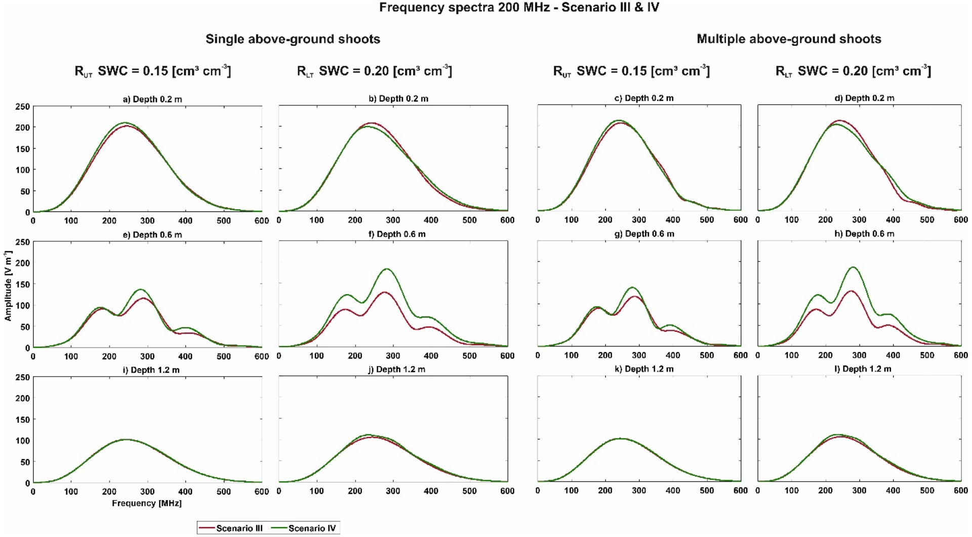
𝜀r results for Scenario III and IV for RUT and RLT and a SWC of 0.15 cm and 0.20 (cm3⋅cm−3), respectively. The error between the input 𝜀r and the modeled 𝜀r is provided in brackets.
| RUT | RLT | |||
|---|---|---|---|---|
| Scenario III | Scenario IV | Scenario III | Scenario IV | |
| SWC | 0.15 | 0.20 | ||
| 𝜀r in the homogeneous half space | 9.62 | 10.78 | ||
| Multiple above-ground shoots | ||||
| 0.1 | 5.05 (−47.52%) | 5.06 (−47.33%) | 5.38 (50.08%) | 5.38 (−50.08%) |
| 0.2 | 8.66 (−9.92%) | 8.94 (−7.07%) | 9.50 (11.89%) | 9.83 (−8.79%) |
| 0.4 | 9.62 (0.0%) | 10.03 (4.26%) | 10.74 (0.32%) | 12.64 (17.25%) |
| 0.6 | 9.62 (0.0%) | 10.00 (4.0%) | 10.74 (0.32%) | 13.67 (26.83%) |
| 0.8 | 9.62 (0.0%) | 9.76 (1.49%) | 10.74 (−0.32%) | 12.97 (20.32%) |
| 1.2 | 9.62 (0.0%) | 9.59 (0.25%) | 10.74 (−0.32%) | 11.00 (2.04%) |
Three-phase soil water content for Scenario III and three-phase and four-phase soil water content results for Scenario IV for RUT and RLT and different SWC conditions 0.15 and 0.20 (cm3⋅cm−3). The % error between the three- and four-phase SWC is provided in brackets.
| RUT | RLT | |||||
|---|---|---|---|---|---|---|
| Scenario III | Scenario IV | Scenario III | Scenario IV | |||
| SWC | 0.15 (cm3⋅cm−3) | 0.20 (cm3⋅cm−3) | ||||
| SWC (three-phase) | SWC (three-phase) | SWC (four-phase) | SWC (three-phase) | SWC (three-phase) | SWC (four-phase) | |
| Single above-ground shoot | ||||||
| 0.1 | 0.07 | 0.07 | 0.04 (−50.68%) | 0.08 | 0.07 | 0.07 (−10.0) |
| 0.2 | 0.16 | 0.16 | 0.13 (−19.14%) | 0.17 | 0.18 | 0.18 (−1.68%) |
| 0.4 | 0.18 | 0.19 | 0.16 (−16.40%) | 0.20 | 0.24 | 0.23 (−1.69%) |
| 0.6 | 0.18 | 0.19 | 0.16 (−15.96%) | 0.20 | 0.25 | 0.25 (−1.18%) |
| 0.8 | 0.18 | 0.18 | 0.15 (−16.85%) | 0.20 | 0.24 | 0.24 (−1.65%) |
| 1.2 | 0.18 | 0.18 | 0.15 (−16.67%) | 0.20 | 0.20 | 0.20 (−1.45%) |
| Multiple above-ground shoots | ||||||
| 0.1 | 0.08 | 0.08 | 0.05 (−43.21%) | 0.09 | 0.09 | 0.08 (−7.87%) |
| 0.2 | 0.16 | 0.17 | 0.14 (−18.56%) | 0.18 | 0.19 | 0.18 (−1.62%) |
| 0.4 | 0.18 | 0.19 | 0.16 (−16.40%) | 0.20 | 0.24 | 0.23 (−1.69%) |
| 0.6 | 0.18 | 0.19 | 0.16 (−15.96%) | 0.20 | 0.25 | 0.25 (−1.18%) |
| 0.8 | 0.18 | 0.18 | 0.15 (−16.85%) | 0.20 | 0.24 | 0.24 (−1.65%) |
| 1.2 | 0.18 | 0.18 | 0.15 (−16.67%) | 0.20 | 0.20 | 0.20 (−1.45%) |
Appendix C. Wave propagation for depth 0.6 m depth Scenario I and II
Image plots (a–d) for Scenario I and (e–h) for Scenario II of the forward modeled electrical field distributions through the model domain for four time steps when the Tx and Rx are located at 0.6 m depth in the RLT with a SWC of 0.1 (cm3⋅cm−3).