


 CC-BY 4.0
1. Introduction
This research article concludes a series published in the Comptes Rendus (Deguen et al., 2024; Nataf and Schaeffer, 2024; Vidal, Noir, et al., 2024; Plunian et al., 2025), sparked by the Ampère Prize awarded in 2021 by the French Academy of Sciences to the géodynamo research team1 . The latter was originally formed to study convective flows within the Earth’s core and the geomagnetic field. Indeed, more than a century after the seminal idea of Larmor (1919), it is well accepted that the geomagnetic field is driven by dynamo action due to turbulent motions in the Earth’s liquid core (e.g. Roberts and King, 2013; Dormy, 2025). Moreover, paleomagnetism indubitably shows that the Earth has hosted a large-scale magnetic field for billions of years (e.g. Macouin et al., 2004). Therefore, the dynamics of the liquid core over geological time scales can be indirectly probed by studying the geomagnetic field. For example, geomagnetic data allows reconstructing surface core flows (e.g. Istas et al., 2023; Rogers et al., 2025), which may enhance future predictions of geomagnetic variations (e.g. Madsen et al., 2025), or anchoring models aimed at understanding the origin of magnetic reversals (e.g. Driscoll and Olson, 2009; Frasson et al., 2025). In addition, understanding the emergence of the geodynamo in the ancient Earth is also of paramount importance, since it would provide invaluable insights into the long-term evolution of the Earth since its accretion (Halliday and Canup, 2023).
1.1. Geologic constraints for dynamo models
Paleomagnetism indicates that the geomagnetic field is at least 3.4–3.5 Gy old (Tarduno, Cottrell, Watkeys, et al., 2010; Biggin, de Wit, et al., 2011), with a paleo-amplitude that is roughly comparable with the present field until −3.25 Gy. Such observations agree well with more indirect estimates from geochemistry. Indeed, the 15 N/14 N isotopic composition of the Archean atmosphere 3.5 Gy ago was found to be rather similar to the one of the present-day atmosphere (Marty et al., 2013), which would require a paleomagnetic amplitude of at least 50% of the current intensity to avoid N2 loss in the upper atmosphere (Lichtenegger et al., 2010). However, planetary scientists currently disagree on whether the Earth’s magnetic field could have appeared earlier or not. It is indeed very challenging to go further back in time, as ancient rocks have experienced multiple geological events throughout their history. As shown in Figure 1, some paleomagnetic studies suggest that the geomagnetic field probably existed during the Eoarchean era with a surface amplitude >15 μT (Nichols, Weiss, et al., 2024), and possibly 4.2 Gy ago as inferred from Hadean silicate minerals (Tarduno, Cottrell, Davis, et al., 2015; Tarduno, Cottrell, et al., 2020; Tarduno, Cottrell, Bono, et al., 2023). However, the quality of such ancient paleomagnetic data is strongly disputed. The magnetic carriers may have a secondary origin, such that the magnetisation could post-date the formation of the minerals by millions to billions of years (e.g. Weiss, Maloof, et al., 2015; Weiss, Fu, et al., 2018; Borlina et al., 2020; Taylor et al., 2023).
Paleointensity at the Earth’s surface during the Hadean and Archean periods. Measurements have been performed on either single-silicate crystals (e.g. zircons) or whole rocks (e.g. Banded Iron Formations). Data from the pint database (Bono, Paterson, et al., 2022) and Nichols, Weiss, et al. (2024). Geological eons are also shown (H: Hadean, A: Archean).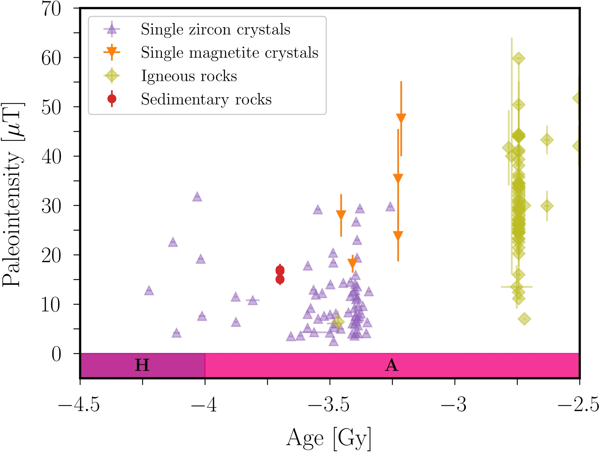
Finding a convincing scenario to explain the ancient Earth’s magnetic field is a long-term goal in geophysical modelling (Landeau, Fournier, et al., 2022). To this end, dynamo action is believed to predominantly operate in the Earth’s liquid core (e.g. Braginsky and Roberts, 1995), as the latter is surrounded by a silicate mantle having a weaker electrical conductivity (compared to that of liquid iron at core conditions) in both its upper and lower regions (e.g. Yoshino, 2010; Jault, 2015, for the Earth). As such, the mantle is often considered as an electrical insulator on long time scales for dynamo modelling. Note that dynamo action may be possible in a (basal) magma ocean if the electrical conductivity of molten silicate rocks is high enough (e.g. Ziegler and Stegman, 2013; Scheinberg et al., 2018; Stixrude et al., 2020; Dragulet and Stixrude, 2025), but this dynamical scenario may be energetically expansive (Schaeffer, Labrosse, et al., 2025). However, there is currently no consensus within the community regarding the physical mechanisms that may have driven core flows in the ancient core.
1.2. Non-consensual dynamo scenarios
To assess the viability of a candidate dynamo scenario, we should strive to reproduce the main characteristics of the recorded field over geological time scales. In particular, we can consider the typical amplitude of the large-scale field in the dynamo region, which can be extrapolated from the data. Indeed, for an electrically insulating mantle, the amplitude Bcmb of the largest-scale dipolar field at the core-mantle boundary (cmb) is related to that at the planet’s surface Bs by (e.g. K. H. Moffatt and Dormy, 2019)
| \begin {equation}\label {eq:Bcmbfromdata} B_{\mathrm {cmb}}\simeq B_s\left (\frac {R_s}{R_{\mathrm {cmb}}}\right )^3, \end {equation} | (1) |
Now, do we have some ancient dynamo scenarios meeting the above constraints? Currently, the main driver of the Earth’s core flows is inner-core crystallisation (e.g. Buffett et al., 1996). Indeed, this scenario has proven successful in reproducing the main characteristics of the current geomagnetic field using numerical simulations (e.g. Schaeffer, Jault, et al., 2017; Aubert, 2023). However, inner-core crystallisation was missing in the distant past. The exact chronology remains disputed, but a nucleation starting 1 ± 0.5 Gy ago seems reasonable from recent thermal-evolution models (e.g. Labrosse, 2015) or paleomagnetism (Biggin, Piispa, et al., 2015; Bono, Tarduno, et al., 2019; T. Zhou, Tarduno, Nimmo, et al., 2022; Y.-X. Li et al., 2023). Prior to inner-core growth, it remains unclear which mechanism could have sustained a large-scale magnetic field. In addition to thermal convection alone (e.g. Aubert, Labrosse, et al., 2009; Burmann et al., 2025; Lin, Marti and Jackson, 2025), various scenarios have been invoked to trigger turbulence in the core (e.g. Landeau, Fournier, et al., 2022), such as flows driven by double-diffusive convection in the core (e.g. Monville et al., 2019) or by tidal forcing (e.g. Le Bars, Cébron, et al., 2015). Indeed, the recent estimates of the thermal conductivity of liquid iron at core conditions, which do not show a consensus yet between experimental and computational values (e.g. Q. Williams, 2018; Hsieh et al., 2025; Andrault et al., 2025), might suggest that secular cooling was energetically less efficient than initially thought to sustain dynamo action in the Earth’s core.
1.3. Outline of the manuscript
Motivated by the paleomagnetic data shown in Figure 1, we want to thoroughly assess whether tidal forcing could have sustained the early Earth’s magnetic field. Landeau, Fournier, et al. (2022) provided preliminary estimates but, as shown below, applying this scenario to the Earth is still intricate. The extrapolation is underpinned by some arguments that must be quantitatively revisited in the light of recent geophysical models and fluid-dynamics studies. Thus, this manuscript also intends to explain how the fluid-dynamic community models tidally driven flows and turbulence in planetary cores.
For instance, to the best of our knowledge, there is no self-consistent numerical code to efficiently explore the dynamo capability of orbitally driven flows in realistic core geometries (i.e. with a weakly non-spherical cmb). This is a noticeable difference with convection-driven dynamos, for which efficient numerical strategies have been developed for decades (e.g. Christensen, Aubert, et al., 2001; Schaeffer, 2013). Therefore, we must currently rely on scaling arguments to extrapolate the few available results to the early Earth. However, planetary extrapolation is not an easy task because it requires a strong understanding of the turbulence properties, which are still debated in the fluid-dynamics community (e.g. as recently reviewed in Vidal, Noir, et al., 2024). Similarly, a universal scaling law that could be applied to any tidally driven flow is unlikely to exist, because the scaling theory should be tailored to each physical mechanism.
With the aforementioned goals in mind, the manuscript is divided as follows. We introduce the basic fluid-dynamics ingredients for core flows driven by orbital forcings (e.g. tides) in Section 2, as they may not be familiar to non-expert readers. We then focus on the tidal forcing in Section 3, combining constraints from geophysical models, hydrodynamic studies and new dynamo scaling laws, to extrapolate our findings to the early Earth. We discuss the results in Section 4, and we end the manuscript in Section 5.
2. Modelling of orbitally driven flows
In this section, we will present the minimal fluid-dynamics ingredients needed to model the dynamics of planetary liquid cores subject to orbital mechanical forcings (such as tides in the early Earth). First, we introduce in Section 2.1 an idealised common description of orbitally driven core flows. Then, we briefly outline in Section 2.2 the different steps of the (expected) flow response of a planetary liquid core to an orbital mechanical forcing, which will be revisited in Section 3 to carry out the planetary extrapolation to the early Earth.
2.1. Equations of fluid dynamics
We want to model the dynamics of a planetary core prior to the nucleation of a solid inner core. Thus, we consider a liquid core of volume V with no inner core, which is surrounded by a rigid and electrically insulating mantle. The cmb is denoted by ∂V below. The core geometry is generally assumed to be spherical in most geodynamo models, as it is sufficient for convection-driven studies and allows developing very efficient numerical methods (e.g. Christensen, Aubert, et al., 2001; Schaeffer, 2013). However, it is important to take the small departures from a spherical cmb into account for tidal and precession forcings (e.g. Le Bars, Cébron, et al., 2015). For simplicity, we assume below that V is an ellipsoid, which agrees with the mathematical theory of equilibrium figures for a rotating fluid mass with an orbital partner (e.g. Chandrasekhar, 1987). Then, it is customary to work in the frame rotating with the ellipsoidal distortion, which is rotating at the angular velocity 𝜴𝜖. Note that the latter generally differs from the rotation of the fluid, which will be denoted by 𝜴s below. Working in the frame rotating at 𝜴𝜖 will ease the computations, since the cmb will be steady in that frame and can be written as (x/a)2 + (y/b)2 + (z/c)2 = 1, where [a,b,c] are the ellipsoidal semi-axes and (x,y,z) are the Cartesian coordinates. Note that dynamical pressure (due to core flows) is expected to be much weaker than hydrostatic pressure on long time scales. Consequently, in practice, the flow dynamics is usually explored in rigid ellipsoids by considering prescribed values of [a,b,c]. Planetary values can be estimated from tidal theory (e.g. Farhat et al., 2022) and the theory of planetary figures (e.g. Chambat et al., 2010). Note that the z-axis is usually chosen along the rotation of the planet, such that it is customary to introduce the two parameters given by
| \begin {equation} \beta = \frac {|a^2-b^2|}{a^2+b^2},\quad f= \frac {a-c}{a}, \end {equation} | (2a,b) |
The core is filled with an electrically conducting liquid, which is assumed to have a constant kinematic viscosity 𝜈 and magnetic diffusivity 𝜂. The ratio of these two quantities yields the magnetic Prandtl number Pm = 𝜈/𝜂, whose typical value is Pm ∼ 10−6 in a planetary liquid core when adopting the typical core values 𝜈 ≃ 10−6 m2⋅s−1 (e.g. de Wijs et al., 1998) and 𝜂 ≃ 1 m2⋅s−1 (e.g. Nataf and Schaeffer, 2024). As a consequence, we expect the magnetic dissipation to be much larger than the viscous one in a dynamo regime. Note that we neglect density effects below, to focus on incompressible fluids with constant density. Indeed, most fluid-dynamics studies consider orbitally driven flows without buoyancy effects in the incompressible regime, assuming that the fluid has a constant density 𝜌f. In the frame rotating at 𝜴𝜖, the fluid velocity v is then governed by the incompressible momentum equations given by
| \begin {eqnarray} \mathrm {d}_t \boldsymbol{v} + 2 {\boldsymbol{\Omega}} _{\epsilon } \times \boldsymbol{v} &=& -\nabla \Pi + \nu \nabla ^2 \boldsymbol{v} + \boldsymbol{f}_L + \boldsymbol{f}_P,\end {eqnarray} | (3a) |
| \begin {eqnarray} \nabla \cdot \boldsymbol{v} &=& 0, \end {eqnarray} | (3b) |
| \begin {equation} \boldsymbol{f}_L = \frac {1}{\rho _f \mu } (\nabla \times \boldsymbol{B}) \times \boldsymbol{B}, \quad \boldsymbol{f}_P = \boldsymbol{r} \times \dot{\boldsymbol{\Omega}}_{\epsilon }, \end {equation} | (4a–b) |
| \begin {eqnarray} \label {eq:induction-a} \partial _t \boldsymbol{B} &=& \nabla \times (\boldsymbol{v} \times \boldsymbol{B}) + \eta \nabla ^2 \boldsymbol{B},\end {eqnarray} | (5a) |
| \begin {eqnarray} \nabla \cdot \boldsymbol{B} &=& 0. \end {eqnarray} | (5b) |
| \begin {equation}\label {eq:BCmag} \boldsymbol{B} = \nabla \Phi ,\quad \Phi \to 0\quad \text {when } |\boldsymbol{r}| \to +\infty . \end {equation} | (6a,b) |
Finally, it is customary to write down the mathematical problem using dimensionless variables. In particular, we introduce the Ekman number E and the Rossby number Ro given by
| \begin {equation} \label {eq:EkRonumbers} E = \frac {\nu }{\Omega _s R_{\mathrm {cmb}}^2},\quad \mathit {Ro} = \frac {\mathcal {U}}{\Omega _s R_{\mathrm {cmb}}}, \end {equation} | (7a,b) |
2.2. Towards dynamo magnetic fields
Even with the strong physical assumptions we have employed, the model presented in Section 2.1 is extremely difficult to solve. One of the reasons is that, currently, there is no numerical code that can efficiently account for magnetic BC (6) in an ellipsoidal geometry. Nonetheless, previous numerical and experimental studies have allowed the identification of a rather general pattern for the flow response to orbital forcings (e.g. Vidal, Noir, et al., 2024, for a recent review). We briefly describe it below, as it will guide us for the extrapolation of tidal forcing in Section 3.
To start with, we consider a non-dynamo regime characterised by negligible magnetic effects, which occurs prior to the establishment of a planetary magnetic field. At the leading order, an orbital forcing drives a large-scale flow U0 in an ellipsoid, which is governed by
| \begin {eqnarray} \mathrm {d}_t \boldsymbol{U}_0 + 2 {\boldsymbol{\Omega}} _{\epsilon } \times \boldsymbol{U}_0 &=& - \nabla \Pi _0 + \nu \nabla ^2 \boldsymbol{U}_0 + \boldsymbol{f}_P,\end {eqnarray} | (8a) |
| \begin {eqnarray} \nabla \cdot \boldsymbol{U}_0 &=& 0. \end {eqnarray} | (8b) |
| \begin {equation} \label {eq:formGP1} \boldsymbol{U}_0 \simeq {\boldsymbol{\Omega}} _{\epsilon } \times \boldsymbol{r} + \nabla \Psi _{\epsilon }, \quad \boldsymbol{U}_0 \cdot \mathbf {1}_n |_{\partial V} = 0, \end {equation} | (9a,b) |
It turns out that the forced laminar flows are unlikely to sustain dynamo action, because their spatial structures are generally too simple (e.g. Tilgner, 1998, for the precession-driven forced flow). However, the flow components departing from U0 could be viable candidates for dynamo action. Indeed, there are often unstable flow perturbations u that can grow upon U0 in the bulk of the core with an amplitude |u|∝ exp(𝜎t) in the initial stage (i.e. when u⋅𝛻u remains negligible in the momentum equation for u), where 𝜎 > 0 is the growth rate of the unstable flows. Physically, such hydrodynamic instabilities can result from couplings between the shear component 𝛻Ψ𝜖 in Equation (9a) and free waves existing in the bulk of the core (e.g. inertial waves, whose restoring force is the Coriolis force associated to the global rotation of the liquid core). The growth rate 𝜎 ⩾ 0 of these unstable bulk flows can be written as
| \begin {equation} \label {eq:growthrateTH} \sigma \simeq \sigma ^i - \sigma ^d, \end {equation} | (10) |
| \begin {equation} \label {eq:sigmaivsdamping} \frac {\sigma ^i}{\Omega _s} > \mathcal {O}(E^{1/2}). \end {equation} | (11) |
After their exponential growth, these flows will saturate in amplitude due to a non-vanishing nonlinear term u ⋅ 𝛻u, and become turbulent. As outlined in Vidal, Noir, et al. (2024), various regimes of turbulent flows can be expected, leading to different scaling laws for the velocity amplitude $\mathcal{U} \sim |\boldsymbol{u}|$ as a function of the control parameters (e.g. E and Ro). Therefore, we need to determine the correct scaling law for the amplitude of turbulence.
Once we can estimate the amplitude of turbulent flows in planetary conditions, we can start assessing their ability to generate a self-sustained magnetic field. In induction equation (5a), the magnetic field can growth over time if the production term 𝛻 × (u × B) is much larger than the dissipation term 𝜂𝛻2B. Using orders of magnitude, this yields the condition that the magnetic Reynolds number Rm, given by
| \begin {equation}\label {eq:Rmnumber} \mathit {Rm} = \frac {\mathcal {U} R_{\mathrm {cmb}}}{\eta } \end {equation} | (12) |
| \begin {equation}\label {eq:Rmcdynamo} \mathit {Rm}_c \sim 40- 100 \end {equation} | (13) |
Finally, the nonlinear regime of orbitally driven dynamos remains unknown. Indeed, direct numerical simulations (dns) of dynamos in ellipsoids have only be performed using either unrealistic (ad-hoc) numerical approximations that strongly hamper the planetary extrapolation (Cébron and Hollerbach, 2014; Vidal, Cébron, Schaeffer, et al., 2018), or were limited to exponential growth regimes (Ivers, 2017; K. S. Reddy et al., 2018). Therefore, we must rely on scaling-law arguments to estimate the possible strength of dynamo fields in planetary interiors. However, there is no consensual dynamo scaling law in the literature for tidal forcing (Le Bars, Wieczorek, et al., 2011; Barker and Lithwick, 2014; Vidal, Cébron, Schaeffer, et al., 2018) or precession (Cébron, Laguerre, et al., 2019).
Finally, it is worth noting that a dynamo scenario can fail at any stage. For instance, condition (11) may not be fulfilled on long enough time scales to yield turbulent flows u, or the resulting turbulence may have not remained vigorous enough to maintain a Rm value above the dynamo onset over time. Similarly, the associated dynamo magnetic field may be too weak to match the paleomagnetic estimates given in Figure 1. Therefore, to assess the dynamo capability of tidally driven flows in the early Earth, we have first to estimate if conditions (11) and (13) are satisfied in the distant past, and then to estimate a typical magnetic field amplitude using appropriate scaling laws.
3. Results for tidal forcing
As customary in long-term evolution scenarios for the Earth–Moon system (e.g. Farhat et al., 2022), we consider a simplified model neglecting the effects of Earth’s obliquity, of the Moon’s orbital eccentricity and inclination, and of the small phase lag between the tidal bulge of the Earth and the Moon. Hence, the Earth’s core is supposed to be instantaneously deformed by the tidal potential into an ellipsoid whose equatorial semi-axes can be written as
| \begin {equation} \frac {a}{R_{\mathrm {cmb}}} = \sqrt {1 + \beta },\quad \frac {b}{R_{\mathrm {cmb}}} = \sqrt {1 - \beta }, \end {equation} | (14a,b) |
Given the above assumptions, tidal forcing first drives a laminar flow in an ellipsoidal liquid core of the form (9) with (e.g. Le Bars, Cébron, et al., 2015)
| \begin {equation} \label {eq:GP1tides} \omega _{\epsilon } = \Delta \Omega \, \mathbf {1}_z, \quad \Psi _{\epsilon } = -\beta \, \Delta \Omega xy, \end {equation} | (15a,b) |
3.1. Estimates from geophysical models
We need to estimate how the geometry of the liquid core has changed over geological time scales, as well as the spin Ωs and the orbital angular velocity Ωorb. It is known that the polar flattening is mainly due to centrifugal effects such that $f \propto \Omega _s^2$ according to equilibrium hydrostatic models (e.g. Chambat et al., 2010). Moreover, tidal theory for an incompressible fluid predicts that the equatorial ellipticity of the core should evolve as 𝛽 ∝ (1/aM)3 (e.g. Cébron, Le Bars, Moutou et al., 2012), where aM is the Earth–Moon distance. Therefore, assuming that the mantle’s properties have not significantly changed over time, the polar flattening f(𝜏) and equatorial ellipticity 𝛽(𝜏) of the core at age 𝜏 before present can be estimated from the present-day values [f(0),𝛽(0)] as
| \begin {equation} \label {eq:betaftime} \frac {f(\tau )}{f(0)}=\left (\frac {\Omega _s(t)}{\Omega _s(0)}\right )^2, \quad \frac {\beta (\tau )}{\beta (0)}=\left (\frac {a_M(0)}{a_M(\tau )}\right )^3, \end {equation} | (16a,b) |
We have to estimate the present-day values [f(0),𝛽(0)], before extrapolating [f(𝜏),𝛽(𝜏)] back in time. Following Chambat et al. (2010), the current flattening f(0) can be obtained using hydrostatic equilibrium theory, with
| \begin {equation} f(0) \approx 2.54 \times 10^{-3} \end {equation} | (17) |
| \begin {equation}\label {eq:betaradius} \beta (0) \simeq \frac {3}{2} \frac {s_{\mathrm {max}}(R_{\mathrm {cmb}})} {R_{\mathrm {cmb}}} \approx 9.8 \times 10^{-8}. \end {equation} | (18) |
Sketch (not to scale) of the elliptical geometry of the tidally deformed Earth’s core, as seen the orbital plane of the Moon. Rs is the mean surface radius, and Rcmb is the mean core radius. The radial displacement along the major axis in the equatorial plane is smax, and that along the minor axis is given by smin = −smax/2 for a tidal potential of degree 2.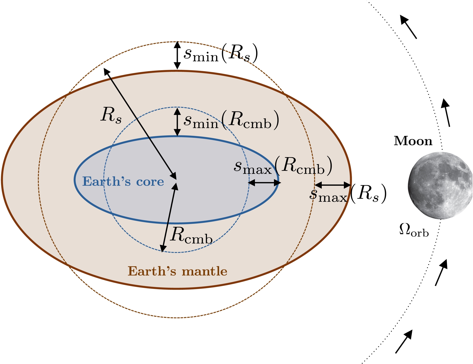
Maximum radial displacement smax and inverse polar flattening f−1 at present day, as a function of normalised mean radius r/Rs, as computed for tidal theory and hydrostatic equilibrium theory. In both cases, the same Earth’s reference model is chosen (Dziewonski and Anderson, 1981). Red region shows the solid inner core, and grey one the liquid outer core.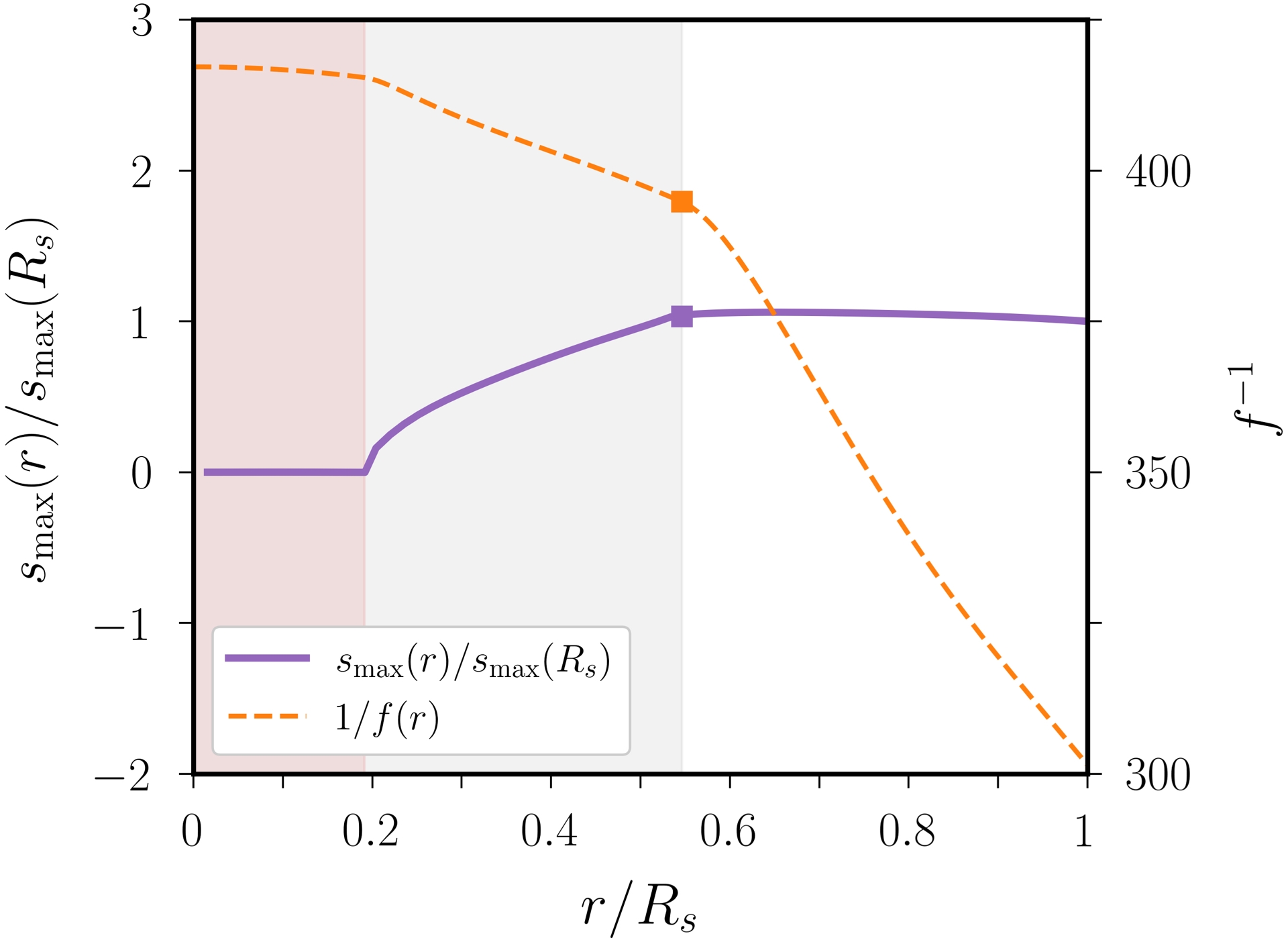
Comparison between geologic data and models for the evolution of the normalised Earth–Moon distance aM/Rs in (a), and of the length of day in (b). Insets show the age 𝜏 between −1 and −0.1 Gy. Rs ≃ 6378 km is the mean value of the Earth’s radius. Orbital model: Farhat et al. (2022). Paleontological data: G. E. Williams (2000) and references therein. Cyclostratigraphic data: M. Zhou, H. Wu, et al. (2024) and references therein. Tidal rhythmites data: Farhat et al. (2022), Eulenfeld and Heubeck (2023) and references therein.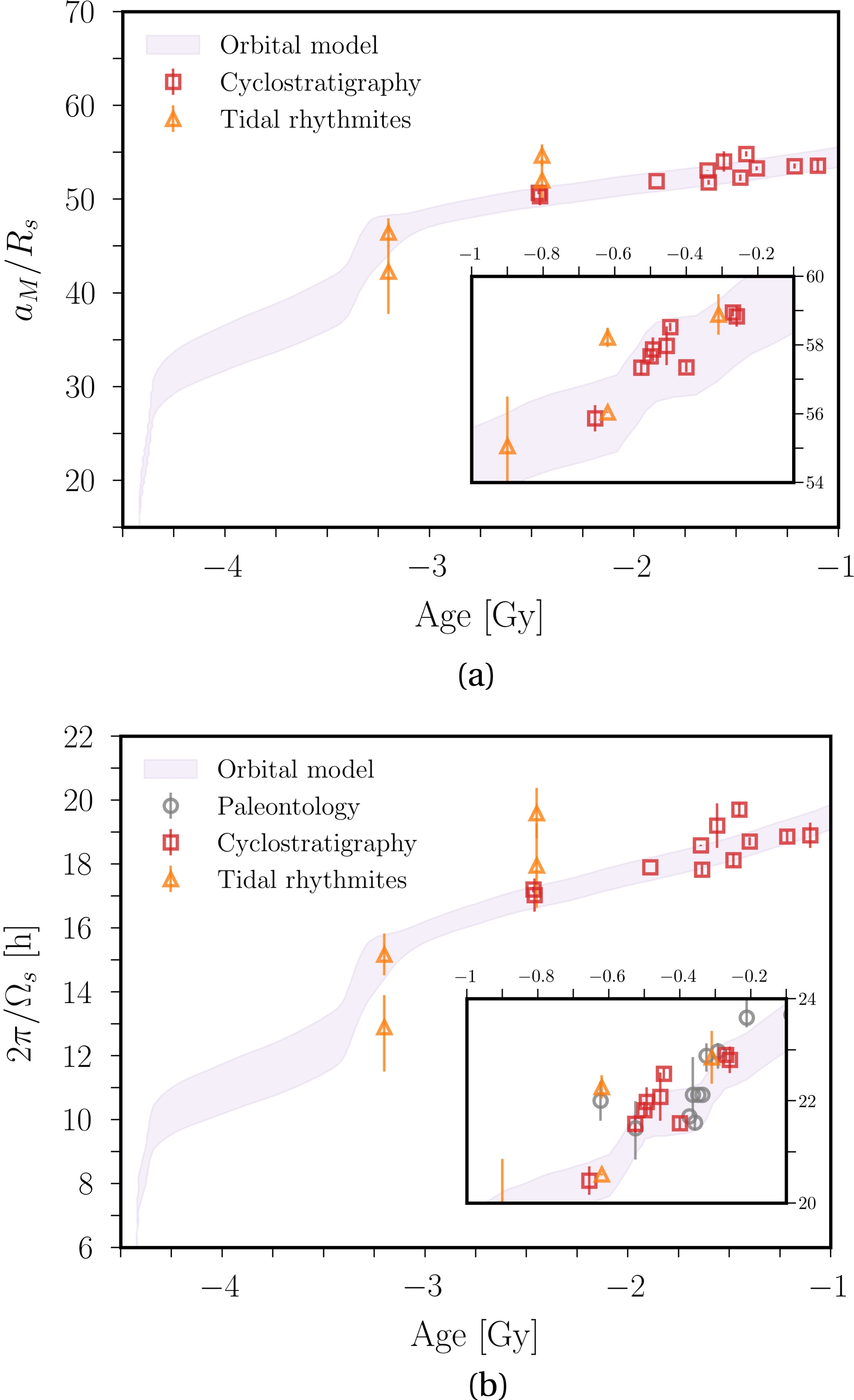
The corresponding values of 𝛽(𝜏) and f(𝜏), computed as a function of 𝜏 from Equations (16a,b), are shown in Figure 5. We see that 𝛽 only varies from one order of magnitude over the Earth’s history, that is from 𝛽 ≈ 10−7 nowadays to 𝛽 ≈ 10−6 at −4.25 Gy. This narrow range of values will put severe constraints for the viability of the tidal scenario (as explained below in Section 3.2). Finally, the Moon’s orbital frequency is reconstructed using Kepler’s third law as
| \begin {equation} \label {eq:kepler3law} \frac {\Omega _{\mathrm {orb}}(\tau )}{\Omega _{\mathrm {orb}}(0)} = \left (\frac {a_M(0)}{a_M(\tau )}\right )^{3/2}, \quad \Omega _{\mathrm {orb}}(\tau )=\frac {2\uppi }{T_{\mathrm {orb}}(\tau )}, \end {equation} | (19a,b) |
Evolution of the Earth’s core ellipticity 𝛽, polar flattening f, and of Ωorb/Ωs, as a function of age. Dashed line shows the frequency value associated with the least-damped mode in resonance condition (20). Geological eons are also shown (H: Hadean, A: Archean, P: Proterozoic).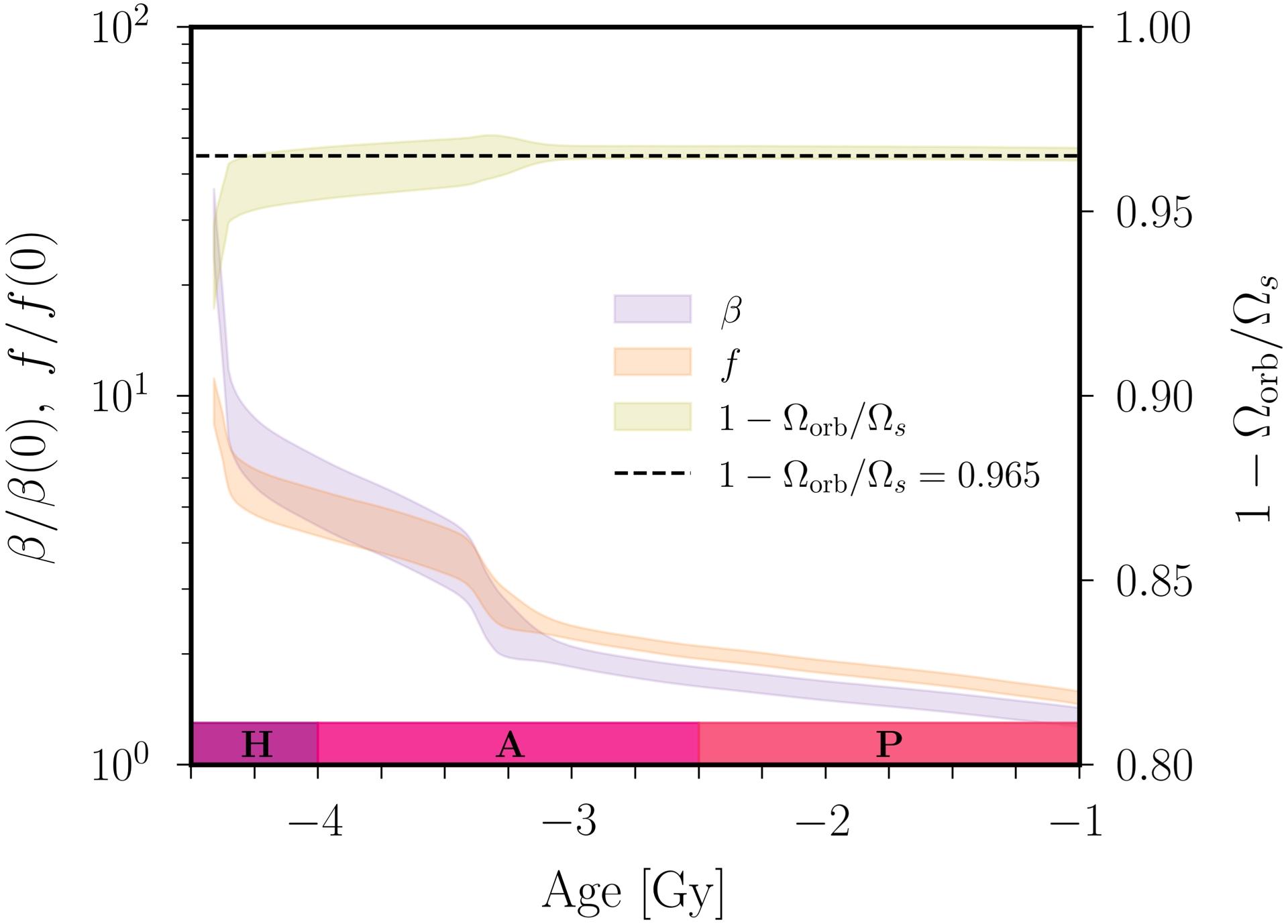
3.2. Hydrodynamic constraints
The geophysical models discussed above have allowed us to estimate the parameters that need to be prescribed in the fluid-dynamics models. Hence, we can move on the hydrodynamic constraints we have about tidal flows. Before we can estimate the strength of dynamo action in Section 3.3, we need to estimate whether turbulent tidal flows could have been triggered in the early Earth’s core in Section 3.2.1 and estimate their amplitude in Section 3.2.2.
3.2.1. Onset of turbulent flows
As outlined in Section 2.2, unstable tidal flows can possibly grow upon the flow U0 with an exponentially increasing amplitude ∝exp(𝜎t) in the initial stage. The underlying mechanism is that of a sub-harmonic (parametric) instability, known as the elliptical instability (Kerswell, 2002; Le Bars, Cébron, et al., 2015). This instability results from couplings between some normal modes ui sustained by the global rotation of the core, called inertial modes and oscillating with an angular frequency 𝜔i, and the shear component of the forced flow U0 through the linearised term (ui⋅𝛻)U0 + (U0⋅𝛻)ui in the momentum equation.
For this instability to exist, the modes and the tidal forcing must satisfy a resonance condition in time given by (e.g. Vidal and Cébron, 2017)
| \begin {equation}\label {eq:resonancecondition} \omega _i \simeq \pm |\Omega _s-\Omega _{\mathrm {orb}}|. \end {equation} | (20) |
| \begin {equation}\label {eq:sigmatdei} \frac {\sigma ^i}{\Omega _s} \lesssim \frac {(2 \tilde {\Omega } + 3)^2} {16(1+\tilde {\Omega })^2} |1 - \Omega _0| \beta \end {equation} | (21) |
| \begin {equation}\label {eq:dampingBLT} \sigma ^{\nu }\simeq \Omega _s (\sigma ^{\nu }_{1/2}\,E^{1/2} + \sigma ^{\nu }_{1}\,E), \end {equation} | (22) |
Equation (22) is illustrated in Figure 6(a). Note that the inertial modes can be expressed in terms of polynomial functions of degree ⩽n in rotating ellipsoids (e.g. Backus and Rieutord, 2017; Colin de Verdière and Vidal, 2025), such that they can be computed using dedicated numerical methods (e.g. Vidal and Colin de Verdière, 2024). We have only shown the modes for which we could expect resonances from condition (20), that is with |𝜔i| ∼ 0.96 ± 0.02 for the early Earth according to Figure 5. Interestingly, we deduce that no modes of degree n < 7 could be triggered in the early Earth’s core. Indeed, the first modes that possibly satisfy resonance condition (20) in the early Earth are the two n = 7 modes whose angular frequencies are
| \begin {equation} \frac {\omega _i}{\Omega _s} \approx \pm 0.965. \end {equation} | (23) |
| \begin {equation} \frac {\sigma ^{\nu }_{1/2}}{\Omega _s} \approx 5.73, \quad \frac {\sigma ^{\nu }_{1}}{\Omega _s} \approx 261. \end {equation} | (24) |
| \begin {equation}\label {eq:dampingTDEIEarlyEarth} {\sigma ^d}/{\Omega _s} \geq 5.73\,E^{1/2} + 261\,E. \end {equation} | (25) |
(a) Surface and bulk contributions to the viscous damping 𝜎𝜈, as a function of the polynomial degree n of inertial modes with 𝛽 = 10−6 and f = 10−2. Only the modes with 0.94 ⩽ |𝜔i/Ωs| ⩽ 0.98 that could satisfy resonance condition (20) are shown. (b) Diffusionless growth rate 𝜎i/Ωs of unstable tidal flows as a function of time, given by formula (21), and leading-order damping term 𝜎d ≳ 𝜎𝜈 as a function of the typical length scale of expected unstable flows. We have used the standard value 𝜈 = 10−6 m2⋅s−1 of the core viscosity (e.g. de Wijs et al., 1998). We have included the prior lower bound obtained with $\sigma ^{\nu }_{1/2}/\Omega _s =2.62$ (blue region). Geological eons are also shown (H: Hadean, A: Archean, P: Proterozoic).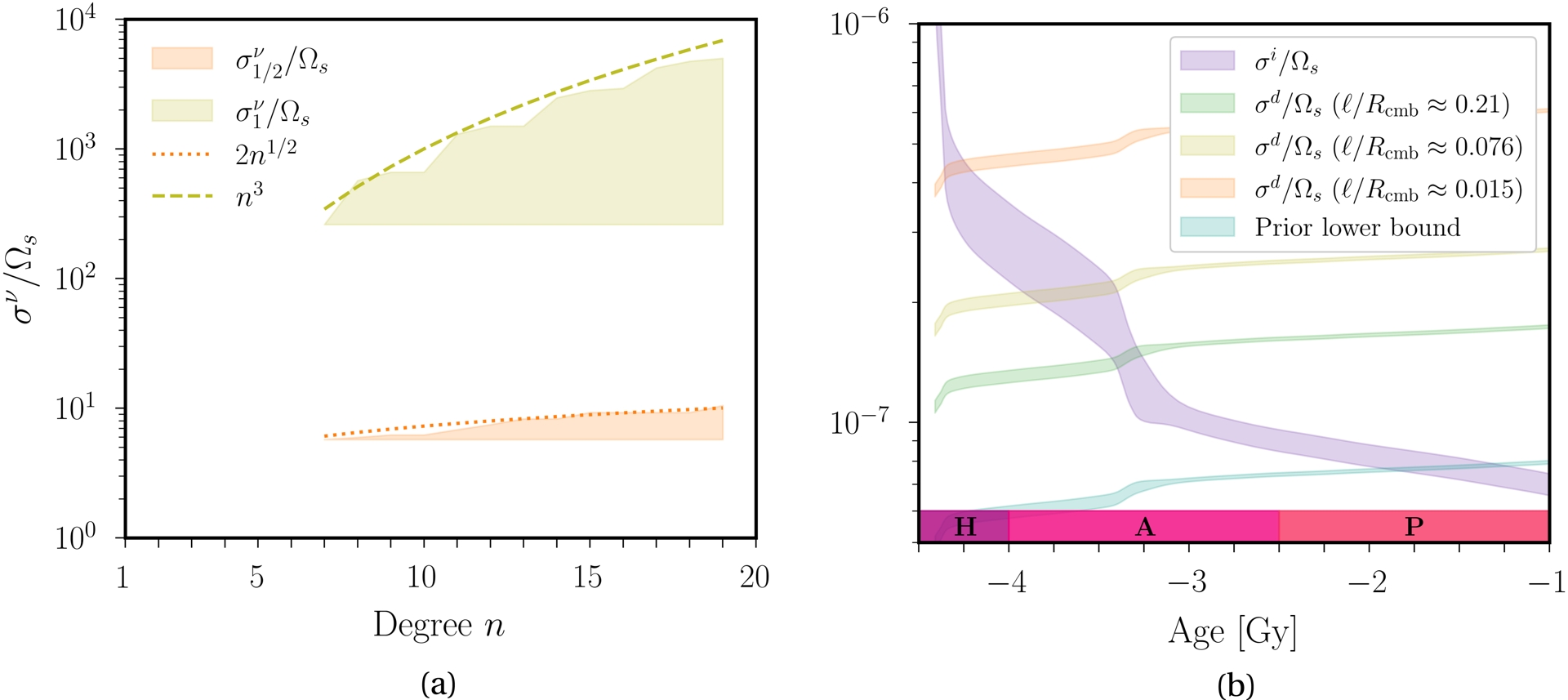
Next, we compare 𝜎i given by Equation (21) and 𝜎𝜈 in Figure 6(b). We have estimated 𝜎𝜈 from Figure 6(a) for unstable flows with the typical length scale ℓ(n) estimated as (Nataf and Schaeffer, 2024)
| \begin {equation}\label {eq:lton} \frac {\ell }{R_{\mathrm {cmb}}} \simeq \frac {1}{2}\frac {\uppi }{n+1/2}, \end {equation} | (26) |
3.2.2. Turbulent flows
Linear analysis yields predictions for the time window where turbulent flows may be triggered by elliptical instabilities (sustained by tidal forcing). Now, we have to estimate the typical velocity amplitude $\mathcal{U}$, as this quantity will play an important role in the planetary extrapolation. To do so, we can have a look at simulations of tidally driven flows without magnetic fields. Actually, several turbulence regimes can be expected. Weakly nonlinear analysis shows that the normal form of the elliptical instability is that of a supercritical Hopf bifurcation (Knobloch et al., 1994; Kerswell, 2002). Hence, the saturation amplitude should scale as $\mathcal{U}/(|\Delta \Omega | a) \propto \sqrt{\beta - \beta _c}$ near the onset, where 𝛽c is the critical ellipticity (i.e. such that 𝜎 = 0). On the contrary, we expect $\mathcal{U}/(|\Delta \Omega | a) \propto \beta - \beta _c \sim \beta $ far enough from the onset according to phenomenological arguments (Barker and Lithwick, 2014).
We estimate $\mathcal{U}$ below from the volume average of the axial velocity component uz, which has been reported in prior numerical and experimental studies. Since we have U0⋅1z = 0, any departure from zero will be associated to tidally driven turbulence and mixing. Moreover, it is often assumed to be a good proxy for the mixing in the core driven by tides, which is key dynamo action driven by tides (e.g. Vidal, Cébron, Schaeffer, et al., 2018). We show in Figure 7 the normalised velocity amplitude $\mathcal{U}$, obtained from simulations in ellipsoids with a rigid boundary at E = 1.5 × 10⁻⁵ and |1 − Ωorb/Ωs| ≈ 1.98 (Grannan et al., 2017). We do recover the two expected regimes in the simulations. The transition is believed to occur when $\beta - \beta _c \sim \mathcal{O}(E)$ from theory (Kerswell, 2002). This is again in broad agreement with the simulations, but we report here a quite large numerical pre-factor since it occurs at 𝛽 − 𝛽c ∼ 600 E. The second regime with 𝛽 ≫ 𝛽c can be more efficiently probed by relaxing the no-penetration BC in the model. This can be achieved by using a free-surface condition in an ellipsoid (Barker, 2016a), or by performing simulations of turbulent flows growing upon U0 in Cartesian periodic boxes (Barker and Lithwick, 2014). Such simulations, performed for different values of E and forcing frequencies |1 − Ωorb/Ωs|, are gathered in the inset of Figure 7. Although they have been performed for different parameters, almost all simulations are well reproduced by the linear scaling law uz/(|ΔΩ|a) ∝ (0.25 ± 0.15) 𝛽 in the second regime (see the inset in Figure 7).
Normalised velocity $\mathcal{U}/(|\Delta \Omega | a)$ with ΔΩ = Ωs − Ωorb, as a function of 𝛽 − 𝛽c (with 𝛽c ≈ 10−2) in dns of tidally driven flows in rigid ellipsoids (Grannan et al., 2017). Inset also shows the velocity but as a function of 𝛽 when 𝛽 ≫ 𝛽c for additional simulations in ellipsoids with a free-surface condition (Barker, 2016a), and in Cartesian boxes (Barker and Lithwick, 2014). In the latter case, we have defined $a = \sqrt{1+\beta }$ for the normalisation. Coloured region shows scaling law $\mathcal{U}/(|\Delta \Omega | a) = (0.25 \pm 0.15)\, \beta $, which broadly agrees with simulations.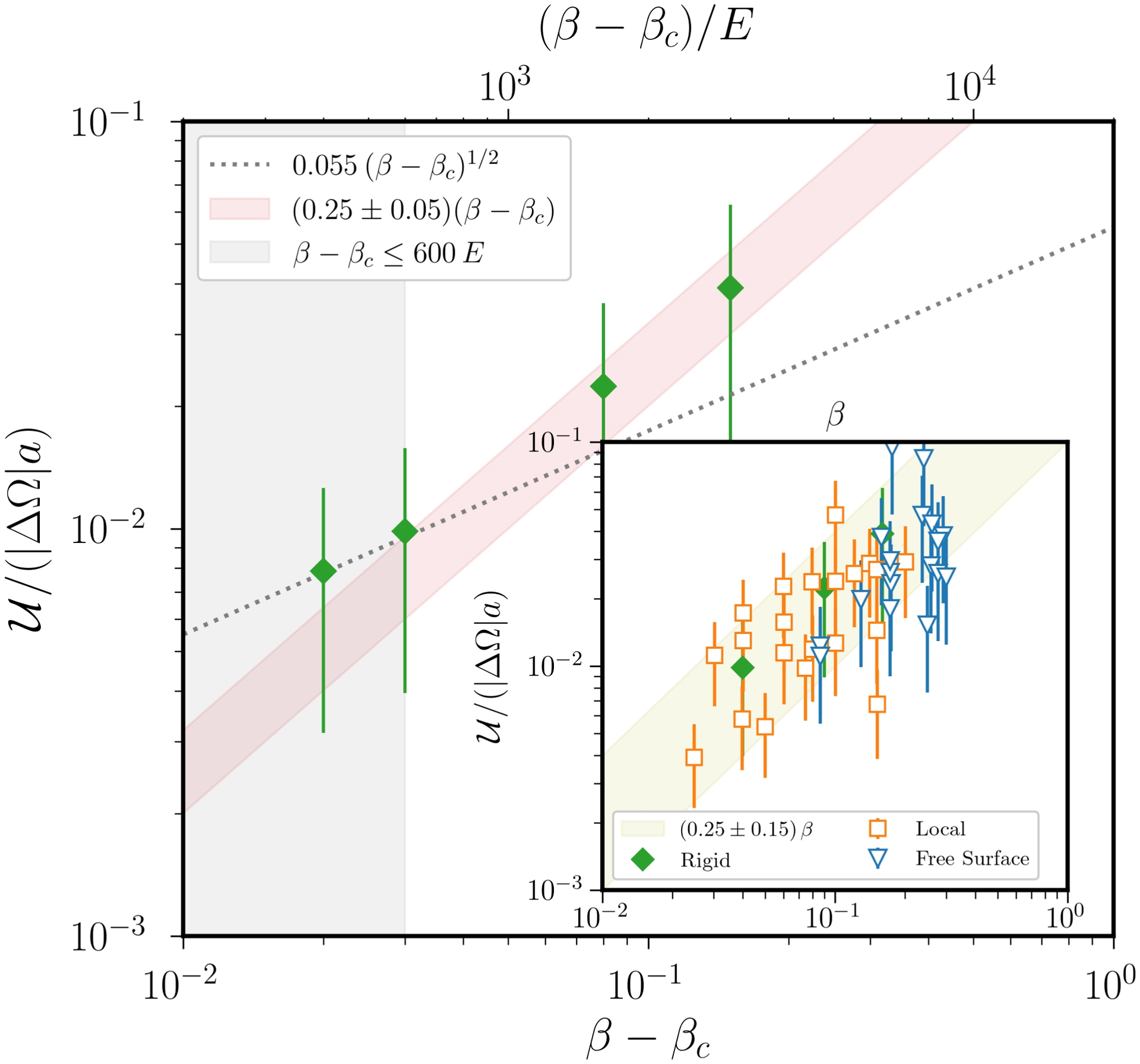
To apply these results to the early Earth, we need to estimate how supercritical the early Earth’s core was before −3.25 Gy. Going back to Figure 6(b), we see that super-criticality is never very large (i.e. 𝜎i/𝜎𝜈 ≪ 10). We can estimate a lower bound for the critical value of the ellipticity at the onset from Equations (21) and (25). This yields
| \begin {equation} \beta _c \gtrsim \frac {5.73\,E^{1/2}}{|1 - \Omega _{\mathrm {orb}}/ \Omega _s|}\frac {16(1+\tilde {\Omega })^2}{(2\tilde {\Omega }+3)^2}, \end {equation} | (27) |
Assuming that the transition between the two regimes still occurs at 𝛽 − 𝛽c ∼ 600 E when E ≪ 1, the early Earth’s core would have been in the second regime for most of the Hadean and Archean eons (since 𝛽 − 𝛽c ≫ 600 E). Therefore, we can consider that the tidally driven velocity amplitude (in planetary cores) is given by
| \begin {equation} \label {eq:scalinglawUtides} \mathcal {U} \simeq \alpha _1 \beta |\Delta \Omega | R_{\mathrm {cmb}}, \quad \alpha _1 = 0.25 \pm 0.15, \end {equation} | (28a,b) |
Finally, we point out that scaling law (28) says almost nothing about the characteristics of the underlying turbulence. Indeed, the properties of tidally driven turbulence remains largely disputed for planetary conditions (e.g. Vidal, Noir, et al., 2024). Scaling law (28) may apply for tidally driven flows characterised by weakly nonlinear interactions of three-dimensional waves when Ro ≪ 1 (Le Reun, Favier, Barker, et al., 2017; Le Reun, Favier and Le Bars, 2019; Le Reun, Favier and Le Bars, 2021), as well as with strong geostrophic flows when Ro ≳ 10−2 (e.g. Barker and Lithwick, 2014; Barker, 2016a; Vidal, Cébron, Schaeffer, et al., 2018).
3.3. A dynamo scaling law
Given the scaling law for the velocity amplitude, we evaluate in Figure 8 the value of Rm, defined in Equation (12), as a function of time. We have chosen a critical value Rmc = 100 for the onset of dynamo action, which is standard in dynamo studies. Our results show a more pessimistic view than the one presented in Landeau, Fournier, et al. (2022), in which the Rm values seem overestimated due to the chosen upper bound value 𝛼1 = 1 in the velocity scaling law. Indeed, taking all uncertainties into account (e.g. on 𝛼1 in the scaling law), we see that the Rm value is rather loosely constrained during most of the Hadean and Archean eons. The uncertainties in the Earth–Moon model yield Rm values that can vary by a factor 2, and those in scaling law (28) even yield more larger variations. As such, tidally driven dynamo action might have well never existed or ceased −4.25 Gy ago, or even have operated until the flow turbulence ceased near −3.25 Gy. Therefore, a putative tidally driven dynamo was likely less super-critical than previously thought. Smaller Rm values not only narrow the time window for a tidally driven dynamo, but also weaken the magnetic field possibly sustained by such a mechanism. In particular, since the amplitude of the tidal forcing decreases over time (see Figure 6b), Rm–Rmc decreases during the Hadean and Archean eons. Hence, we expect the magnetic field driven by tidal forcing to weaken over time. This may be at odds with the paleomagnetic measurements shown in Figure 1(a), which may suggest that the (maximum) amplitude of the geomagnetic field did not vary much between −3.5 and −2.5 Gy. In the following, we focus on dynamo action during the late Hadean and Archean eras (where more powerful tidally driven dynamos may be expected).
Magnetic Reynolds number Rm as a function of age 𝜏. Second y-axis shows the amplitude $\mathcal{U}$ of the expected turbulence according to formula (28) when 𝜏 ⩽ − 3.25 Gy. Gray zone shows the non-dynamo region Rm ⩽ Rmc with Rmc = 100. Predictions younger than −3.25 Gy are hidden, since the elliptical instability was not triggered (see Figure 6b). Prior bound from Landeau, Fournier, et al. (2022) has been included for comparison. Geological eons are also shown (H: Hadean, A: Archean).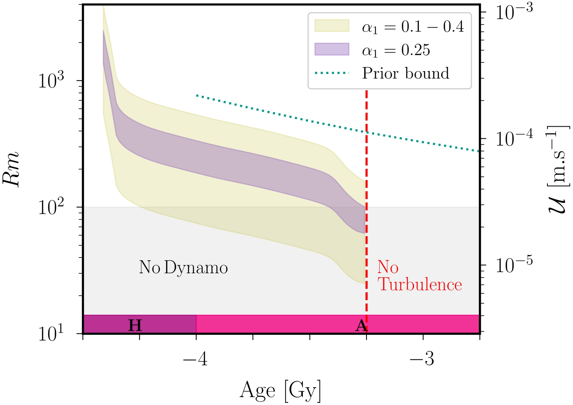
Since state-of-the-art dns cannot properly investigate dynamo action for realistic cmb geometries and in geophysical conditions (even for convective flows in spherical geometries), appropriate scaling laws must be developed to establish a connection between dynamo modelling and geophysical parameters. We assume that Rm–Rmc was large enough at that time, to render the proposed scaling laws for dynamo action in the vicinity of the onset invalid (e.g. Fauve and Pétrélis, 2007). A fruitful approach in dynamo theory is to consider power-based scaling laws (Christensen and Aubert, 2006; Christensen, 2010; Davidson, 2013). For convection-driven dynamos, such laws are often tested against numerical results regardless of the parameters (e.g. Oruba and Dormy, 2014; Schwaiger et al., 2019), and have provided useful insight into planetary extrapolation. In such scaling theories, the saturated magnetic energy density per unit of mass, which is given by
| \begin {equation}\label {eq:MagNRJ} \mathcal {E}(\boldsymbol{B}) = \frac {1}{\rho _f V} \int _V \frac {\boldsymbol{B}^2}{2 \mu }\,\mathrm {d}V \sim \frac {1}{2} \frac {B^2}{\rho _f \mu } \end {equation} | (29) |
| \begin {equation}\label {eq:epsilon_eta} \epsilon _{\eta } = \frac {1}{\rho _f V} \int _V \frac {\eta }{\mu } |\nabla \times \boldsymbol{B}|^2\,\mathrm {d}V \sim \frac {\eta }{\rho _f \mu } \frac {B^2}{\ell _B^2}, \end {equation} | (30) |
| \begin {equation}\label {eq:lawBdavidson} B \propto \sqrt {\rho _f \mu }\, (R_{\mathrm {cmb}} \mathcal {P}_M)^{1/3}. \end {equation} | (31) |
Next, could we faithfully use scaling law (31) for tidally driven dynamos? Since there are no dynamo simulations of tidal flows in ellipsoids against which we can compare theoretical predictions, we cannot be assertive. However, we expect the above power-based arguments to remain largely valid for orbitally driven flows. We have re-analysed in Figure 9 magnetohydrodynamics simulations of tidally driven flows performed in Cartesian periodic boxes at Ro ≳ 10−2 (Barker and Lithwick, 2014). Note that it was not possible to separate 𝜖𝜈 and 𝜖𝜂 in the re-analysis of the published magnetohydrodynamic simulations. Yet, a good agreement is found with scaling law (31), assuming that $\mathcal{P}_M \sim \epsilon _{\nu } + \epsilon _{\eta }$ in a statistically steady state. Such observations are very promising, but quantitative applications to planets remain somehow speculative at present for tidal forcing. Indeed, it is difficult to safely estimate $\mathcal{P}_M$ for geophysical conditions.
Simulations of tidally driven flows at moderate values of Ro, performed in Cartesian periodic boxes of unit length L at Pm = 1. Data from Barker and Lithwick (2014). Typical magnetic field amplitude B defined from Equation (29), as a function of total dissipation 𝜖 = 𝜖𝜈 + 𝜖𝜂.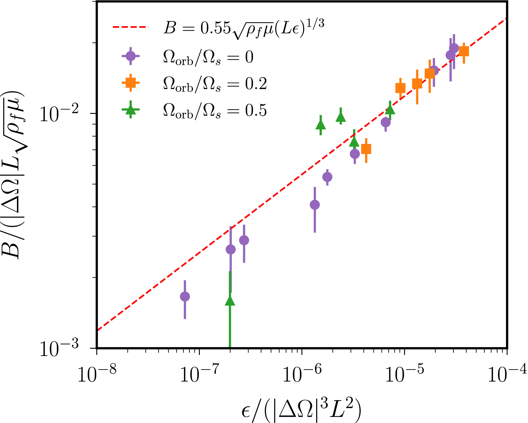
3.4. Towards planetary conditions
We have found that dynamo scaling law (31) is likely valid for tidally driven flows. However, it remains difficult to apply this law in practice, because tidally driven turbulence is still poorly understood at planetary core conditions. To make progress in this direction, we first present in Section 3.4.1 the arguments that underpin our planetary extrapolation in Section 3.4.2.
3.4.1. Heuristic rationale
We can further analyse the dynamo simulations presented in Figure 9, as they can guide us for the planetary extrapolation below. Indeed, these simulations were performed for moderate values of the Rossby number Ro ≳ 10−2, for which scaling arguments have been proposed in rotating turbulence. In such a regime, rotating turbulence usually exhibits strong nearly two-dimensional (geostrophic) flows (e.g. Le Reun, Favier and Le Bars, 2019; Le Reun, Gallet, et al., 2020). Two different scaling theories have been proposed when Ro ≲ 1, such that that the mean viscous dissipation could either scale as (Nazarenko and Schekochihin, 2011; Baqui and Davidson, 2015)
| \begin {equation} \epsilon _{\nu } \sim \frac {u^3_{\ell _{\parallel },\ell _{\perp }}} {\ell _{\perp }} \quad \text {or}\quad \epsilon _{\nu } \sim \frac {u^3_{\ell _{\parallel },\ell _{\perp }}} {\ell _{\parallel }}, \end {equation} | (32a,b) |
| \begin {equation}\label {eq:epsU3/ltides} \epsilon _{\nu } \sim \frac {\mathcal {U}^3}{\ell } \propto \beta ^3 \end {equation} | (33) |
Simulations of tidally driven flows at moderate values of Ro, performed in Cartesian periodic boxes of unit length L at Pm = 1. Data from Barker and Lithwick (2014). Total dissipation 𝜖𝜈 + 𝜖𝜂 as a function of equatorial ellipticity 𝛽. Inset shows the magnetic field amplitude as a function of 𝛽.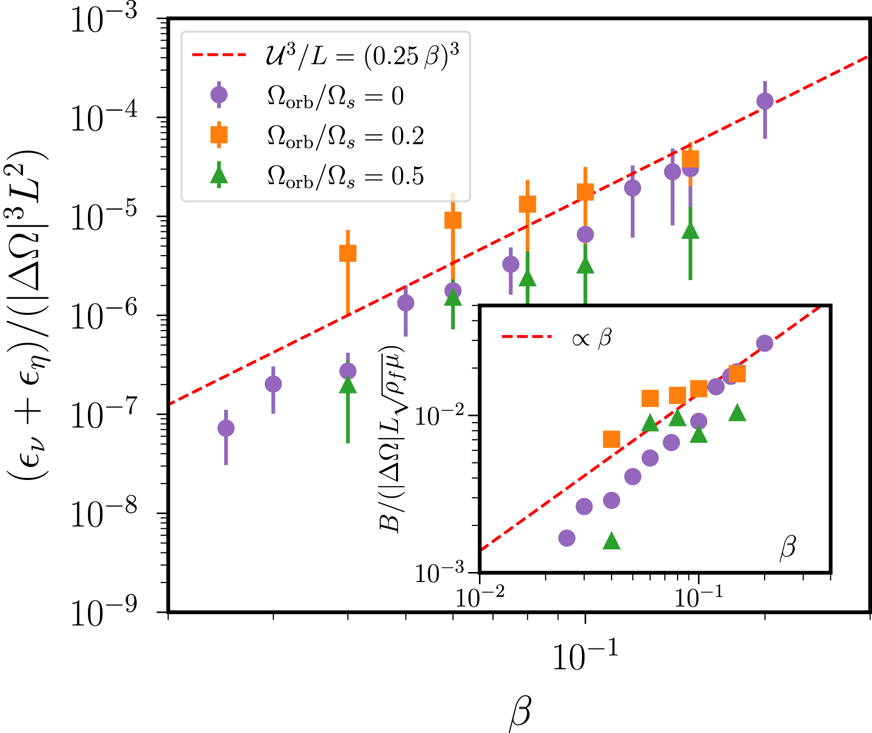
These results show that, for planetary extrapolation, the injected power $\mathcal{P}_M$ for dynamo action can be estimated from the bulk dissipation sustained by the turbulent flows in a statistically steady state. Moreover, the theoretical prediction laws could hold in a dynamo regime by considering the total dissipation (instead of the viscous one). Such heuristic findings are consistent with the fact that, in the nonlinear regime, the elliptical-instability mechanism involves inertial-wave motions. Indeed, inertial waves are barely affected by magnetic effects in realistic core conditions, and are such that $\mathcal{E}(\boldsymbol{B})/\mathcal{E}(\boldsymbol{u})<1$. This results from the dispersion relation of magnetohydrodynamic waves in unbounded fluids (e.g. K. H. Moffatt and Dormy, 2019), and have also been obtained numerically in an ellipsoid (Vidal, Cébron, ud-Doula, et al., 2019; Gerick, Jault, et al., 2020). It is also worth noting that mean-field dynamo theory shows that turbulent interactions of inertial waves could sustain weak-field dynamo action (H. K. Moffatt, 1970a; H. K. Moffatt, b). Therefore, we assume below that inertial wave motions play a key dynamical role in sustaining a weak-field dynamo regime driven by tidal forcing, which will allow extrapolating our theoretical laws to the Earth.
3.4.2. A plausible extrapolation
The regime Ro ≲ 1 described above could apply to short-period Hot Jupiters (e.g. Barker and Lithwick, 2014; Barker, 2016a) or binary systems (e.g. Vidal, Cébron, ud-Doula, et al., 2019), in which tidal forcing can be much stronger such that large values 𝛽 → 10−2 could be obtained. On the contrary, the Earth’s core is characterised by much smaller values Ro ∼ 10−7–10−6. For such small values Ro ≪ 1, tidal forcing is believed to sustain a regime of inertial-wave turbulence (Le Reun, Favier, Barker, et al., 2017; Le Reun, Favier and Le Bars, 2019; Le Reun, Favier and Le Bars, 2021). This is a regime of weak turbulence, characterised by weakly nonlinear interactions of three-dimensional inertial waves. Like in Kolmogorov turbulence, inertial-wave turbulence involves energy being injected at some large scale, denoted by ℓ below. This energy is then transmitted to smaller scales via a direct cascade in an inertial range, in which the input power is balanced by dissipation at every scale, until energy is finally dissipated at sufficiently small scales at a rate 𝜖. However, contrary to isotropic homogeneous turbulence, inertial-wave turbulence is described by an anisotropic energy spectrum (Galtier, 2003; Galtier, 2023), depending on the two length scales ℓ∥ ⩾ ℓ⊥ introduced above.
By analogy with the regime Ro ≲ 1 described in Section 3.4.1, we assume that the injected power $\mathcal{P}_M$ available for dynamo action can be estimated in a statistically steady state from the dissipation 𝜖 of turbulent flows given by wave-turbulence theory when Ro ≪ 1. This rests on the fact that inertial waves are barely modified by magnetic effects at core conditions, such nonlinear interactions of almost pure inertial waves will still be triggered in a weak-field dynamo regime. The main difference with the pure hydrodynamic regime would be that, for small values Pm ≪ 1, the dissipation would occur on a diffusive magnetic length scale larger than the viscous one, such that the width of the inertial range (in the wavenumber space) would be shortened compared to the hydrodynamic case. Hence, we estimate the effective dissipation as (Galtier, 2003; Galtier, 2023)
| \begin {equation}\label {eq:IWT} \epsilon _{\mathit {Ro} \ll 1} \sim \frac {\ell _{\parallel }}{\ell _{\perp }} \frac {u_{\ell _{\parallel },\ell _{\perp }}^4}{\Omega _s\ell _{\perp }^2} \end {equation} | (34) |
Figure 6(b) shows that tidal forcing can only inject energy at rather large scales ℓ (i.e. at fraction of the core radius denoted by 𝛼2 below), for which we may assume ℓ⊥∼ ℓ∥∼ ℓ. Moreover, scaling law (28) shows that $u_{\ell _{\parallel }, \ell _{\perp }} \lesssim \mathcal{U}$ at large scales. Altogether, this allows us to estimate the mean dissipation in a regime of inertial-wave turbulence as
| \begin {equation}\label {eq:IWT2} \epsilon _{\mathit {Ro} \ll 1} \lesssim \frac {\mathcal {U}^4}{\Omega _s \ell ^2} \end {equation} | (35) |
Finally, we can combine Equations (33)–(35) with dynamo scaling law (31) to obtain
| \begin {equation}\label {eq:BIWTtides} B \propto \sqrt {\rho _f \mu } \begin {cases} \alpha _2^{-1/3}\,\mathcal {U} & \text {if } \mathit {Ro} \lesssim 1\\ \alpha _2^{-2/3}\,\mathit {Ro}^{1/3} \mathcal {U} & \text {if } \mathit {Ro} \ll 1 \end {cases} \end {equation} | (36) |
| \begin {equation} B \propto \begin {cases} \beta & \text {if } \mathit {Ro} \lesssim 1\\ \beta ^{4/3} & \text {if } \mathit {Ro} \ll 1 \end {cases} \end {equation} | (37) |
| \begin {equation} \mathcal {E}(\boldsymbol{B})/\mathcal {E}(\boldsymbol{u}) \propto \begin {cases} \alpha _2^{-2/3} & \text {if } \mathit {Ro} \lesssim 1\\ \alpha _2^{-4/3}\,\mathit {Ro}^{2/3} & \text {if } \mathit {Ro} \ll 1. \end {cases} \end {equation} | (38) |
The predictions from scaling law (36) as a function of the age are illustrated in Figure 11. We obtain as a typical estimate B ∼ 10−5–10−3 mT during the Hadean period 4.25–4 Gy ago (i.e. when tidal forcing was maximal), and the field amplitude would then ultimately decrease until −3.25 Gy (since tidal forcing had a decreasing amplitude during the Archean era). The predicted amplitudes are thus at least ten times smaller than the cmb field Bcmb, which is estimated from surface measurements with Equation (1). Therefore, it seems unlikely that the ancient geodynamo was solely sustained by a wave-turbulence regime at Ro ≪ 1 driven by tidal forcing.
Paleointensity at the cmb Bcmb, reconstructed Figure 1 using Equation (1) with Rs = 6378 km and Rcmb = 3480 km, and upper bounds for B (dotted and dashdot lines) from scaling law (36) when Ro ≪ 1. Numerical estimates using 𝜌f ≃ 1.1 × 10⁴ kg⋅m−3 for a mean density (accounting for the mass of the outer and inner cores), 𝜂 = 1 m2⋅s−1, and 𝜇 = 4π × 10−7 H⋅m−1. Geological eons are also shown (H: Hadean, A: Archean).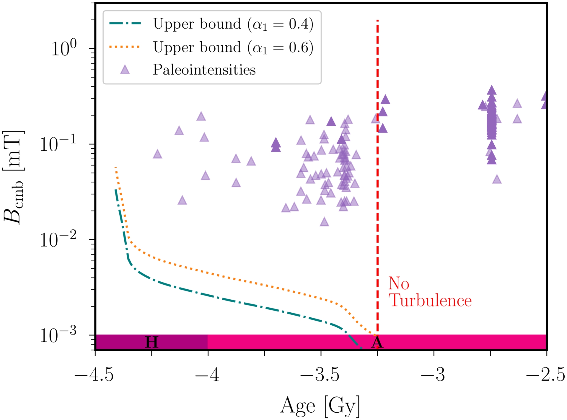
4. Geophysical discussion
Our extrapolation suggests that tidal forcing may have been too weak to generate a dynamo magnetic field with an amplitude matching the (scarce) Hadean and Archean paleomagnetic measurements, at least for flows in a wave-turbulence regime. Since several assumptions were made to arrive at this conclusion, we discuss below if our main results could be modified or not by adopting other modelling choices.
4.1. Influence of the orbital scenario
Obviously, one source of uncertainty arises from the parameters given by the orbital scenario, which was less constrained in the distant past. We have here employed the semi-analytical model by Farhat et al. (2022), as it fits most of the available geological proxies for the history of the Earth–Moon system and reproduce the age of the Moon’s formation fairly well. However, we should assess how the results could be affected by adopting other orbital scenarios. Most models reasonably well agree on the recent Earth–Moon evolution (i.e. after −1 Gy), as they are constrained by geological data. However, the models can significantly differ further back in time.
The comparison between different orbital models is shown in Figure 12. Note that we have discarded models that cannot be extrapolated during the Hadean and the Archean eras (e.g. Green et al., 2017; Zeeden et al., 2023; M. Zhou, H. Wu, et al., 2024). We find that the presented models fall within the error bars of the model by Farhat et al. (2022). This is probably due to the conservation of angular momentum that is enforced in all the models, which gives good constraints on the Earth–Moon distance for a given value of the Earth’s spin rate. Yet, the evolution curves can differ in time between the models. In particular, the model by Tyler (2021) does not reproduce the estimated age of the Moon, overestimating the Earth–Moon distance during the Hadean and Archean eras. A similar conclusion can be drawn for Daher et al. (2021), as shown in Figure 6 of Eulenfeld and Heubeck (2023). On the contrary, the model by Touma and Wisdom (1994) is found to be quite close to the orbital model by Farhat et al. (2022). Consequently, our results already account for most of the uncertainties of the community regarding the orbital scenario. However, the next generation of orbital models may change the overall picture.
Uncertainties in the orbital model. Comparison between the predictions in the distant past from different orbital models (Touma and Wisdom, 1994; Tyler, 2021; Farhat et al., 2022) for the Earth–Moon distance aM/Rs and the length of day. Inset is analogous to Figure 4(a), and to Figure 6 in Eulenfeld and Heubeck (2023). Geological eons are also shown (H: Hadean, A: Archean, P: Proterozoic).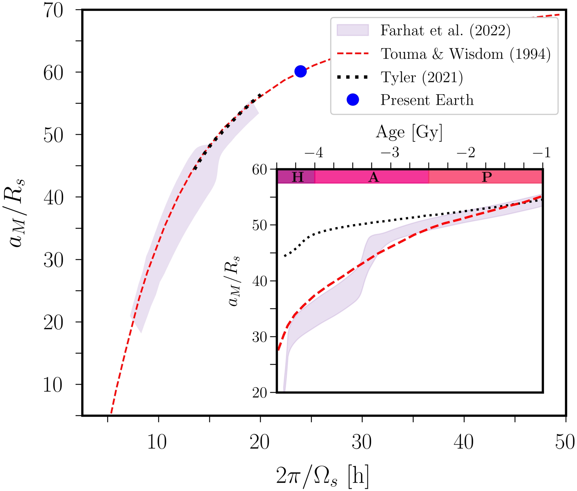
4.2. Rheological uncertainties
Another key quantity in the model is the present-day value of the equatorial ellipticity 𝛽(0) at the cmb. Seismological observations of the peak-to-peak amplitude of the cmb topography (e.g. Koper et al., 2003; Sze and van der Hilst, 2003) suggest that the current value of the equatorial ellipticity may be order-of-magnitude larger than our considered value in Equation (18). However, as this elliptical deformation results from mantle dynamics, it is nearly in phase with the spin frequency of the Earth (i.e. ΔΩ ≈ 0). As such, we do not expect this elliptical deformation to play a role in the elliptical-instability mechanism. This is only the asynchronous component of the ellipticity, which is driven by tidal forcing, that is able to drive an elliptical instability inside the liquid core. The amplitude of the tidal potential is quite well constrained at the present time Agnew (2015), such that the main uncertainties on the value of 𝛽(0) probably come from the mantle’s rheology.
We have employed the prem model (Dziewonski and Anderson, 1981) to account for the Earth’s rheology in Figure 3. More recent Earth models could naturally be used together with the open-source code TidalPy (Renaud, 2023), but this is beyond the scope of the present study. More importantly, we have assumed that the mantle remained rigid over time. This seems to be a reasonable assumption throughout most the Earth’s history, but the Earth’s mantle was probably molten after the giant impact that formed the Moon (at least partially, e.g. Nakajima and Stevenson, 2015). Then, a crystallising basal magma ocean (bmo) probably survived in the aftermath for millions of years to a billion of years (e.g. Labrosse et al., 2007; Boukaré et al., 2025). How such a bmo could have interacted with tidal forcing remains largely unknown (e.g. Korenaga, 2025a; Korenaga, 2025b; Korenaga, 2025c), as well as its possible interactions with core flows. A crude extrapolation of old fluid-dynamics experiments on the spin-up of rotating immiscible fluids (Pedlosky, 1967; O’Donnell and Linden, 1992) might suggest that cmb dissipation is not significantly reduced in the presence of a low-viscosity bmo (due to interfacial friction with the core, and Ekman friction with the solid mantle above). However, further work is needed to elucidate this question.
4.3. Early core’s conditions remain elusive
In addition to the orbital parameters and mantellic properties, there are also uncertainties regarding the physical state of the liquid core in the distant past. In particular, additional dissipation mechanisms may have operated within the core, hindering the onset of tidally driven turbulence over geological timescales.
4.3.1. Hydrodynamic dissipation in the core
The value of the core’s viscosity 𝜈 appears to be another physical quantity of interest when determining the occurrence of tidally driven turbulence. Indeed, as shown in Figure 6, it controls the leading-order damping inhibiting the growth of unstable flows. We have chosen the standard value 𝜈 = 10−6 m2⋅s−1 (e.g. de Wijs et al., 1998), but the core value may be between 10−7 m2⋅s−1 and 3 × 10⁻⁶ m2⋅s−1 (Mineev and Funtikov, 2004). Thus, in Figure 6, the damping term may be decreased by a factor of $\sqrt{10} \approx 3$ with the lowest value, or increased by a factor $\sqrt{3} \approx 2$ with the largest one. Similar effects could be obtained if the liquid core were rotating in the bulk faster or slower than the mantle. We have here assumed that the liquid core is co-rotating with the mantle at the angular velocity Ωs, but the core may be rotating a bit faster than the mantle according to some tidal models (e.g. Wahr et al., 1981). Our model would then remain largely unchanged, except that the value of E would be smaller as it must be based on the fluid rotation (see in Greenspan, 1968).
Note that possible interactions between tidal forcing and buoyancy effects, such as with either convective flows or density stratification, could also provide additional dissipation mechanisms in the core. Convection would essentially sustain slowly varying flows in the core, whereas tidal forcing may mainly trigger high-frequency motions with inertial-wave turbulence. Because of this separation of time scales, strong interactions are not expected between both flows (unless convective flows could locally cancel out the rotation of the core, e.g. de Vries et al., 2023a; de Vries et al., b). Convection would then provide an additional damping, but the latter might be rather weak for fast tidal forcing (e.g. Duguid et al., 2020a; Duguid et al., b; Vidal and Barker, 2020a; Vidal and Barker, b). Note that the early core may have been instead (at least partially) stably stratified in density, according to thermal evolution modelling (only for large values of the thermal conductivity of liquid iron at core conditions, e.g. Labrosse, 2015) or if the early core had been insufficiently mixed after giant impacts (Landeau, Olson, et al., 2016). In this case, density stratification would not modify the largest growth rate of the elliptical instability 𝜎i (Vidal, Cébron, ud-Doula, et al., 2019). Similarly, boundary-layer theory suggests that the value of the damping rate would not change much with a stable density stratification (Friedlander, 1989), such that the predictions shown in Figure 6(b) may remain quantitatively accurate. However, preliminary simulations show that density stratification could significantly weaken the strength of radial flows and mixing (Vidal, Cébron, Schaeffer, et al., 2018). We may thus expect dynamo action to be less favourable with stratification, but further work is needed to carefully investigate the interplay with density stratification.
4.3.2. What about magnetic damping?
It is unclear whether the early core was subject to strong magnetic effects during the Hadean era, that is before an undoubted dynamo action was recorded in paleomagnetic data. However, the Earth’s core had a magnetic field since from at least −3.5 Gy, whatever its dynamical origin. Hence, we may wonder if the presence of an ambient magnetic field (possibly of different origin) could alter the onset of tidally driven flows within the core during the Archean era.
Actually, the elliptical-instability mechanism would be largely unchanged in the presence of a background field. To quantify magnetic effects, we usually introduce the Lehnert number defined as
| \begin {equation} \mathit {Le}=\frac {B_{\mathrm {cmb}}}{\Omega _s R_{\mathrm {cmb}}\sqrt {\rho _f\mu }}. \end {equation} | (39) |
4.4. Scaling-law uncertainties
The presented tidal scenario heavily relies on different scaling laws, which must be used to extrapolate the results in the turbulent regime to core conditions. We have done our best to constrain the various scaling laws as much as possible, by uniquely combining an Earth–Moon evolution scenario with theoretical results and re-analyses of the most up-to-date numerical simulations of tidally driven turbulent flows. Yet, other modelling uncertainties also call the dynamo extrapolation into question. In particular, the outcome of turbulent tidally driven flows and dynamo action remains uncertain as discussed below.
4.4.1. Comparison with earlier works
We have shown in Figure 8 that the prior predictions presented in Landeau, Fournier, et al. (2022) are likely overestimated, since we have used the same modelling assumptions in our study. This mainly results from the chosen numerical prefactors in the different extrapolation laws, which were set to unity for a first proof-of-concept study.
Notably, we have revisited the value of 𝛼1 in velocity scaling law (28), showing that 𝛼1 = 1 disagrees with the available numerical results gathered in Figure 7. Instead, the numerical simulations suggest that 𝛼1 ≃ 0.25 ± 0.15 for planetary extrapolation. Note that we have estimated the value of $\mathcal{U}$ directly from uz. Actually, we found that |uz|∼ 0.7–0.8 |u| for most of the dynamo simulations presented in Figures 9 and 10, where |u| is estimated from the kinetic energy $\mathcal{E}(\boldsymbol{u})$. This is in good agreement with a preliminary estimate of the radial mixing induced by tidally driven flows (see Figure 4 in Vidal, Cébron, Schaeffer, et al., 2018). However, if the horizontal mixing were also important for dynamo action, the velocity prefactor 𝛼1 may be increased up to 0.6. Yet, this would only lead to a small increase of the magnetic field amplitude (see the dashdot line in Figure 11). Future research work may thus shed new light on this estimate. For instance, it is unknown whether the value of 𝛼1 could be increased or not when E is lowered (and similarly 𝛽) but, heuristically, we always expect 𝛼1 < 1 to sustain tidally driven turbulence in the core over long time scales. Otherwise, tidally driven turbulent flows would become of the same amplitude as the shear component of the forced flow U0 when 𝛼1 → 1, which would temporarily stop the injection of energy and hinder the development of a wave-turbulence regime. This may echo some peculiar regimes in rotating turbulence, which are sometimes observed in experiments involving growth-and-collapse phases (e.g. McEwan, 1970; Malkus, 1989). We might also obtain during the energy growth regimes of self-killing dynamos (e.g. Reuter et al., 2009; Fuchs et al., 1999), which have already been reported in simulations of precession-driven flows in a sphere (Cébron, Laguerre, et al., 2019). If such exotic regimes were obtained, our theoretical predictions for the flow turbulence and its dynamo capability would be invalid.
Finally, there are also strong uncertainties associated with dynamo scaling law (31). Obviously, the lack of numerical methods for simulating self-sustained dynamos in ellipsoids currently hampers our ability to assess its validity for planetary relevant regimes. For instance, the inset of Figure 10 shows that the simulations are compatible with
| \begin {equation} B \approx 0.55 \sqrt {\rho _f \mu }\,(R_{\mathrm {cmb}}\epsilon )^{1/3}, \end {equation} | (40) |
4.4.2. Disputed wave-turbulence regime
We have assumed that tidal forcing establishes a regime of inertial-wave turbulence, as often postulated after Le Reun, Favier, Barker, et al. (2017), Le Reun, Favier and Le Bars (2019; 2021). However, inertial-wave turbulence is a research topic that is far from being well understood, especially because it is very challenging to obtain in simulations or in laboratory experiments. As such, current investigations still strive observing predictions of wave-turbulence theory in set-ups mimicking as much as possible the theoretical model (e.g. Yarom and Sharon, 2014; Monsalve et al., 2020). Therefore, it is still unclear whether the quantitative predictions of wave turbulence theory could be directly applied to rotating turbulent flows in bounded geometries at Ro ≪ 1, such as in the early Earth’s core with Ro ∼ 10−7. On the contrary, Figure 10 shows that simulations at moderate values Ro ∼ 10−2 already agree fairly well with the dissipation law (33).
Moreover, how magnetic effects modify inertial-wave turbulence remains speculative so far. We conjecture that inertial-wave turbulence can persist in a weak-field dynamo regime, since high-frequency inertial waves are barely affected by magnetic fields in an ellipsoid. The main difference would be that the dissipation would occur on a diffusive magnetic length scale for small values Pm ≪ 1. This may agree with the qualitatively view drawn from magnetohydrodynamics simulations of tides (Barker and Lithwick, 2014; Vidal, Cébron, Schaeffer, et al., 2018) and precession (Barker, 2016b; Kumar et al., 2024), showing that the obtained turbulence could be largely unchanged in a weak-field dynamo regime. Future numerical works, for instance using local simulations at smaller values of Pm, may shed new light on this point.
4.4.3. A magnetostrophic dynamo regime?
Apart from wave turbulence, another possibility could be that tidally driven turbulence at Ro ≪ 1 could be in a regime of geostrophic turbulence characterised by the presence nearly two-dimensional (geostrophic) flows. This would challenge the applicability of wave-turbulence theory when Ro ≪ 1 (e.g. Gallet, 2015), since geostrophic flows are filtered out in the wave-turbulence theory. However, a regime of hydrodynamic geostrophic turbulence is likely to be modified by magnetic effects. This notably rests on the properties of low-frequency waves in rotating systems subject to magnetic effects. Indeed, slow quasi-geostrophic wave motions morph into various low-frequency waves shaped by the magnetic field, such as torsional Alfvén waves (e.g. Luo and Jackson, 2022) and magneto-Coriolis waves (e.g. Luo, Marti, et al., 2022; Gerick and Livermore, 2024). Consequently, a magnetostrophic regime is expected to supersede purely geostrophic turbulence when Ro ≪ 1 (e.g. Hollerbach, 1996). In such a regime, the Coriolis force could balance the Lorentz force such that B would be given by (e.g. Christensen, 2010)
| \begin {equation}\label {eq:Bmagnetostrophic} B \propto \sqrt {\rho _f \mu } \sqrt {l_B \Omega _s \mathcal {U}}. \end {equation} | (41) |
5. Concluding remarks
5.1. Summary
We have thoroughly explored the capability of tidal forcing to explain the ancient geodynamo. We have combined geophysical constraints from Earth–Moon evolution models, theoretical predictions, and re-analyses of recent results on tidally driven turbulent flows. This has allowed us to show that tidal forcing was likely strong enough to sustain turbulence prior to −3.25 Gy, and possibly dynamo action. However, the self-sustained magnetic field was certainly too weak to explain paleomagnetic measurements if tides were only sustaining an inertial-wave turbulence regime in the ancient core. We hope that our results will guide future studies of tidally driven flows, to possibly strive beyond the limits we have identified. For example, we outlined that magnetostrophic turbulence driven by tidal forcing might produce a strong-field dynamo consistent with the observations. However, evidence of such a tidally driven regime remains to be found.
Alternatively, other mechanisms in the core could be invoked to explain the ancient geodynamo (see in Landeau, Fournier, et al., 2022). For instance, the cmb heat flow extracted by mantle convection could power thermal convection in the ancient core (e.g. Al Asad and Lau, 2024), but this requires low-to-moderate values of the thermal conductivity of liquid iron at core conditions (e.g. Hsieh et al., 2025; Andrault et al., 2025). Alternatively, exsolution (or precipitation) of light elements below the cmb could sustain double-diffusive turbulent convection in the core (e.g. Monville et al., 2019). Yet, a difficulty with such mechanisms may be to obtain vigorous enough turbulence, or to sustain magnetic fields with a dipolar morphology. Actually, a weak tidally driven dynamo might have been important in providing an optimal magnetic seed of finite amplitude to kick-start an efficient convection-driven geodynamo (Cattaneo and Hughes, 2022).
5.2. Towards precession in the Moon?
Beyond Earth, the Moon is another planetary body for which we have geological samples that could help to understand planetary dynamos over long time scales. The analysis of Apollo samples (Figure 13) has revealed that the Moon had a planetary dynamo field in the distant past (e.g. Wieczorek et al., 2023), with a (possibly intermittent) magnetic activity from about −4.2 Gy until at least −1.9 Gy. Recent analyses confirmed that the Moon was first characterised by a high-field epoch (Lepaulard, Gattacceca, et al., 2019; Jung et al., 2024), which persisted from ∼3.9 until ∼3.5 Gy ago, with measured surface field intensities of 40–110 μT. This high-field period was then succeeded by an epoch with a declining field (Tikoo, Weiss, Cassata, et al., 2014; Strauss et al., 2021), whose surface amplitude fell to below 10 μT after −3.5 Gy. Note that it remains unclear whether a lunar core dynamo was long-lived (e.g. Cai, Qi, et al., 2024; Cai, Qin, et al., 2025), episodic (e.g. Evans and Tikoo, 2022), or instead limited to the first hundred millions of years of the Moon’s life (T. Zhou, Tarduno, Cottrell, et al., 2024). In any case, the magnetic activity certainly ceased between −1.9 and −0.8 Gy (Tikoo, Weiss, Shuster, et al., 2017; Mighani et al., 2020).
Paleointensity at the Moon’s surface, inferred from Apollo rocks. Olive region: high-field dynamo epoch. Old Apollo values extracted from Lepaulard, Gattacceca, et al. (2019).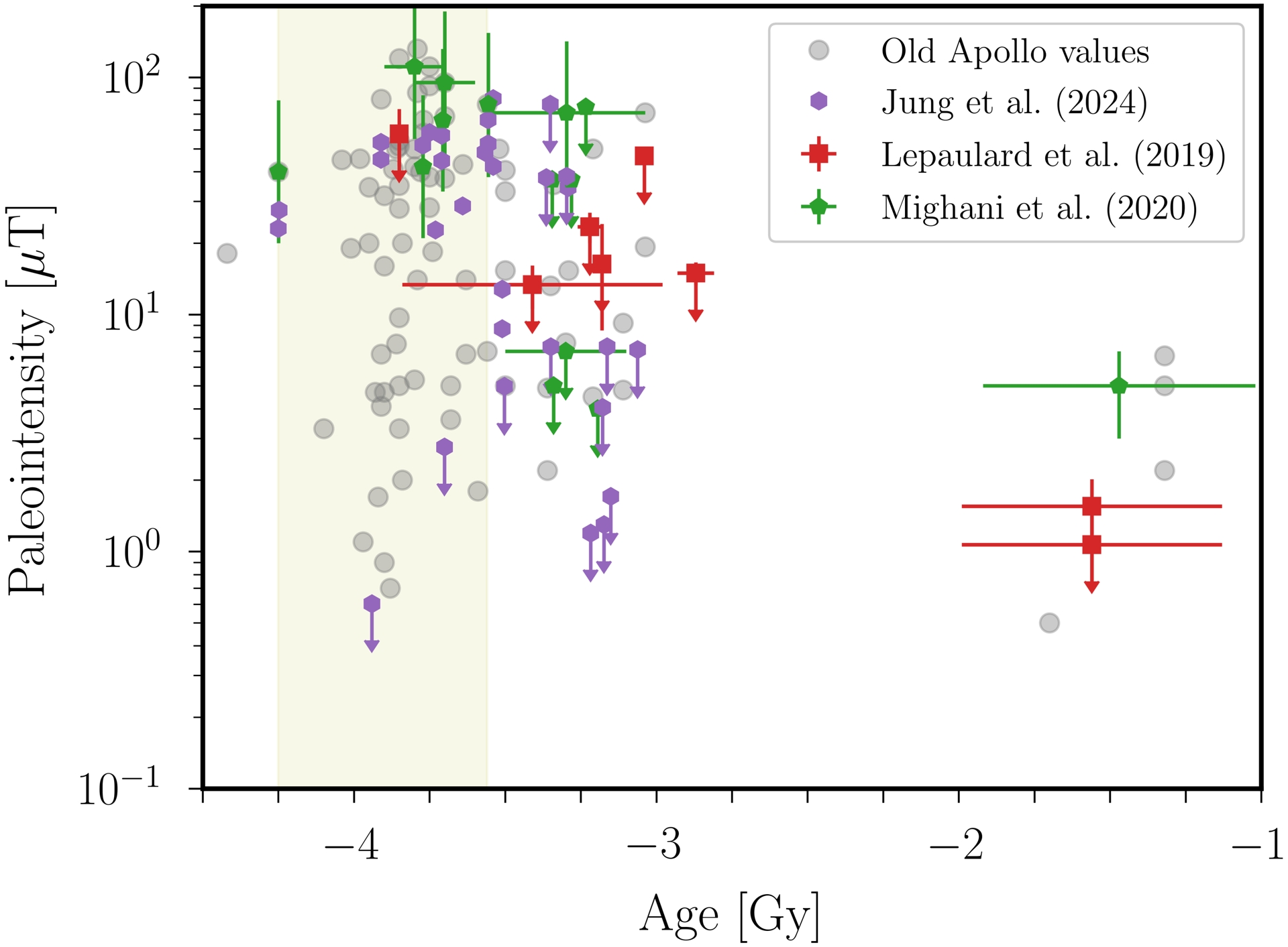
Actually, such paleomagnetic data put very tough constraints for dynamo action inside the ancient Moon. As inferred from Equation (1), any viable dynamo scenario should be capable of generating a magnetic field that is 10 larger in the Moon’s core than in the Earth’s one, despite its core radius being about 10 times smaller (e.g. Bcmb ∼ 10–70 mT during the high-field epoch, with Rcmb ≈ 200–380 km). However, standard dynamo scenarios currently fail to explain the observed field values (Wieczorek et al., 2023). It has been proposed that the ancient Moon’s dynamo could result from precession-driven flows (e.g. Dwyer et al., 2011), which have many dynamical similarities with tidal flows (e.g. Vidal, Noir, et al., 2024). The géodynamo team and its collaborators have worked on precession for a long time, making pioneering contributions to the hydrodynamics (e.g. Noir, Jault, et al., 2001; Lin, Marti and Noir, 2015) and magnetohydrodynamics (Lin, Marti, Noir and Jackson, 2016; Cébron, Laguerre, et al., 2019) of such flows. The present work, at the crossroad of the géodynamo’s research activities, may thus also guide future studies of precession-driven flows.
CRediT authorship contribution statement
Jérémie Vidal: conceptualisation, formal analysis, methodology, software, visualisation, funding, writing—original draft, writing—review and editing.
David Cébron: funding, writing—review and editing. Both authors gave final approval for submission, and agreed to be held accountable for the work performed therein.
Acknowledgements
The authors warmly acknowledge an anonymous referee for the thorough revision of the manuscript, which helped to greatly improve its quality. JV thanks Les Houches School of Physics for the hospitality and stimulating discussions during the workshop “Physics of Wave Turbulence and beyond”, which occurred in September 2024 and where the main idea of the study first emerged. JV also acknowledges the organisers of the Advanced Summer School “Mathematical Fluid Dynamics”, which was held in Corsica in April 2025 and where part of the work was finalised.
Declaration of interests
The authors do not work for, advise, own shares in, or receive funds from any organisation that could benefit from this article, and have declared no affiliations other than their research organisations.
Funding
JV received funding from ens de Lyon under the programme “Terre & Planètes”. DC received funding from the European Research Council (erc) under the European Union’s Horizon 2020 research and innovation programme (grant agreement No 847433, theia project). As part of the géodynamo team, DC greatly acknowledges the support from the French Academy of Sciences & Electricité de France.
Supplementary materials
The matlab code used to compute the Earth’s flattening in Figure 3 is available at http://frederic.chambat.free.fr/hydrostatic/HYDROSTATIC_dec2011.zip. The code TidalPy used to compute the tidal deformations in Figure 3 is available at https://doi.org/10.5281/zenodo.14867405.
1 ISTerre, Université Grenoble Alpes, France, https://www.isterre.fr/english/research/research-teams/geodynamo/.
2 We have 𝜇 ≈ 𝜇0 for core conditions in practice, where 𝜇0 is the magnetic permeability of vacuum.