

1 Introduction
The total mRNAs of genes to test are extracted from the studied tissue (in the present case a glioblastome tissue). DNAs are synthesized by reverse transcription from these mRNAs including bases labelled with the isotope P33. Resulting DNAs are then tested against identified complementary DNAs (cDNA targets), previously amplified by PCR and fixed on a nylon gel. The hybridisation results are revealed in a phospho-imager and yield a digital image coming from the radioactive hybridisation plate, called the bio-array image or shortly the bio-image. cDNA hybridised with a P33DNA means that the complementary sequence of the P33DNA is present in the related mRNA, proving that the corresponding gene is expressed in the studied tissue.
2 Peak segmentation
The first encountered problem is the fact that the bio-images are extremely noisy and that we have to low-pass them in order to suppress the high-frequency noise. The result of this pre-treatment (Fig. 1) is a better separation of the isotopic activity peaks, allowing a watershed separation and contouring [1,2], but it often leads to over-estimating the peak activity.
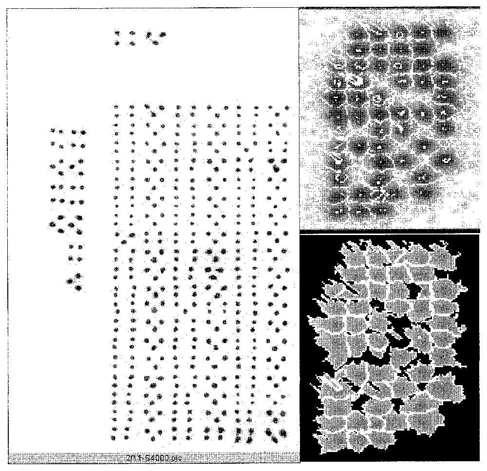
Raw data (left), watershed segmenting (top right), and contouring (bottom right).
Then we will apply a more accurate segmentation and contouring method called the potential-Hamiltonian or ‘Gaussian stamping’ method: let us remark that the peaks are about Gaussian, with a relatively weak kurtosis and skewness allowing in particular the respect of the conservation ‘law’: 2/3 of the peak activity are concentrated into the set of points (x,y) where the Gaussian curvature H(x,y) vanishes, i.e. inside the maximum gradient line of the peak. By exploiting this property, it is possible to neglect the part of the peak outside the projection of this remarkable line, called in the following the characteristic line, its equation being:
We are thus led to consider the new grey function H(x,y) instead of the function g(x,y) and its level line H(x,y)=0. We display after a plane differential system of which the characteristic line is a limit cycle. Let H′(x,y) be the function defined by: H′(x,y)=|H(x,y)|. Vanishing of H′(x,y) occurs on the characteristic line (see Fig. 2 for the visualization of g and H′) and if we consider the following crude system:
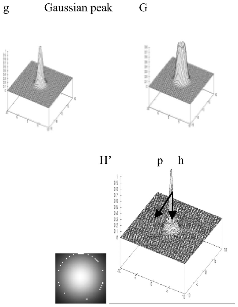
Representation of g, G, H′ (with indication of potential p and Hamiltonian h parts) for a Gaussian peak and the result of the Hamiltonian segmentation (below left).
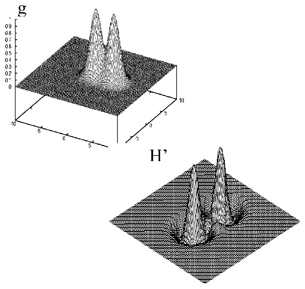
g (top) and H′ (bottom) for close Gaussian peaks.
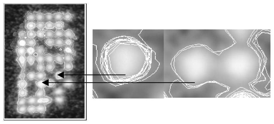
Treated bio-image (left), succeeding limit cycle (middle) and false contour (right).
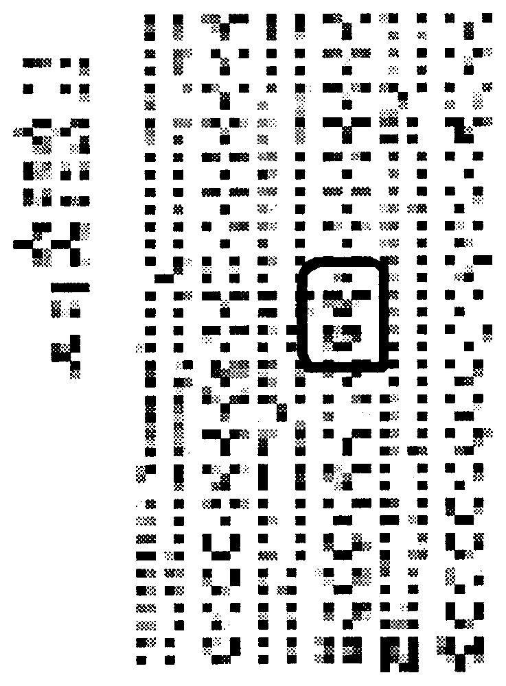
Standardized bio-image (the treated sub-image of Fig. 4 is inside the black rectangle).
3 Interaction matrix
A major problem a geneticist has presently to face since the introduction of the bio-array imaging is the estimation of the intergenic interaction matrix that rules the observed genes expression in operons and genetic regulatory networks [3–7]. This interaction matrix is similar to the synaptic weight matrix, which rules the relationships between neurons in a neural network. Hence, it is in general of a great biological interest and relevance to determine matrices having characteristics like: (i) a minimal number of non-zero coefficients for a given set of stationary behaviours (fixed points or cycles), (ii) a minimal number of positive or negative circuits, controlling the number of attractors and their stability (cf. [8–21] for both the discrete and the continuous case). In this paper, we give some general results about the relationships between the positive and negative circuits in the graph of the interaction matrix and the existence of fixed points. This permits us to characterize minimal matrices, given dynamical behaviours, and therefore partly solve the first problem. Finally, we constructed a bound for the number of fixed points in terms of the number of positive circuits in the graph of the interaction matrix . So we partly solve the second problem too.
In general, it is very difficult to have exhaustively the interaction matrices: in the genetic literature and also by observing co-expressions through bio-arrays imaging, it is possible to qualitatively or even quantitatively estimate the inhibitory (in case of repression by a protein obtained from the expression of a gene) or activatory (in case of induction or promotion) coefficients of the interaction matrix. If we have no information, we can randomly choose the matrix by respecting certain basic rules, e.g., by respecting certain proportions of activatory or inhibitory interactions. We can, for example, obtain the location density of expressed ubiquitory genes (calculated from http://www.citi2.fr/GENATLAS/) and then randomly simulate the interaction matrix and the initial conditions of the gene expression, by sampling them 100 000 times, the interaction matrices respecting the constraint to have 10% (resp. 10%) of negative (resp. positive) interactions, like in the Arabidopsis thaliana genome [3]. Fig. 6 below gives the distribution of the co-expression of the ubiquitory genes calculated from the expected stationary behaviour corresponding to a random choice of the interaction matrix and of the initial conditions: we have systematically calculated attractors (fixed points or limit cycles) corresponding to an initial condition and an interaction matrix, and then we have calculated the frequency of observing the expression of each ubiquitory gene in these attractors. In the absence of complementary information about the localization of the inhibitory or activatory interactions between ubiquitory genes, the obtained co-expression distribution is just a reflect of the spatial distribution of these ubiquitory (domestic or housekeeping) genes along the human chromosome 3 showing that it is related to the rearrangements (due to physiological crossing-over or to pathological translocations) distributions, this parenthood being proved by the analogy between their signatures—i.e. their succession of monotony intervals of increase (+) or decrease (−)—as shown in Table 1.
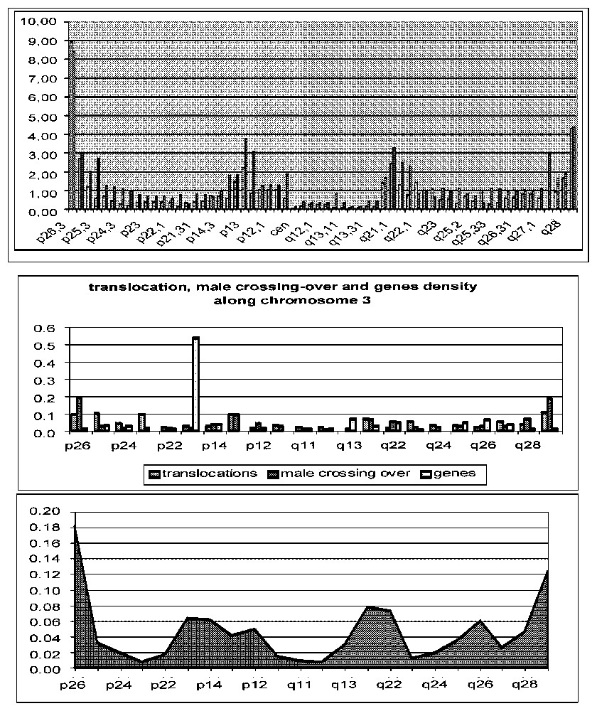
Distributions of domestic (bottom) and all genes (middle right), crossing-over (male red and female blue top) and translocations (middle left) along chromosome 3.
Second column shows the distribution signatures and third the number of differences (− or + being not taken different from =) between a given distribution and the crossing-over one as reference
| Ubiquitory genes distribution | − | − | − | + | + | = | − | + | − | = | = | + | + | = | − | + | + | + | − | + | + | 3/21 |
| All genes distribution | + | = | − | + | + | − | − | + | − | + | = | + | − | + | − | = | + | + | − | − | + | 9/21 |
| Crossing-over distribution | − | = | = | = | = | + | + | − | − | − | = | + | + | − | − | = | = | = | + | + | + | 0/21 |
| Translocation distribution | = | − | + | − | = | = | + | − | + | − | = | = | + | − | + | − | = | = | + | − | + | 3/21 |
By comparing the distribution signatures given in Table 1 above, it is easy to prove that we must reject the hypothesis that ubiquitory genes and translocation distributions are different from the crossing-over distribution (p<0.001), but we cannot reject the hypothesis of a difference between all genes and the crossing-over distribution.
The general coefficient mij of the interaction matrix is equal to +1 if the gene Gj activates the gene Gi, equal to −1 if the gene Gj inhibits the gene Gi and equal to 0 if Gj and Gi have no interaction, Gi being equal to +1 (resp. −1), if it is (resp. not) expressed. Then the change of state xi of the gene Gi between t and t+1 obeys a threshold rule: xi(t+1)=H(∑k=1,nmikxk(t)−bi) or , where H is the sign-step function (H(y)=1, if y⩾0 and H(y)=−1, if y<0) and the bis are threshold values. In the case of small regulatory genetic systems (the smallest being called operons), the knowledge of such a matrix permits to make explicit all possible stationary behaviours of the organisms having the corresponding genome: for example, in the genetic regulatory network that rules the Arabidopsis thaliana flower morphogenesis (Fig. 7), the interaction matrix is a (11,11)-matrix, with only 22 non-zero coefficients. This matrix presents a certain number of positive or negative circuits and only four observed attractors [3].
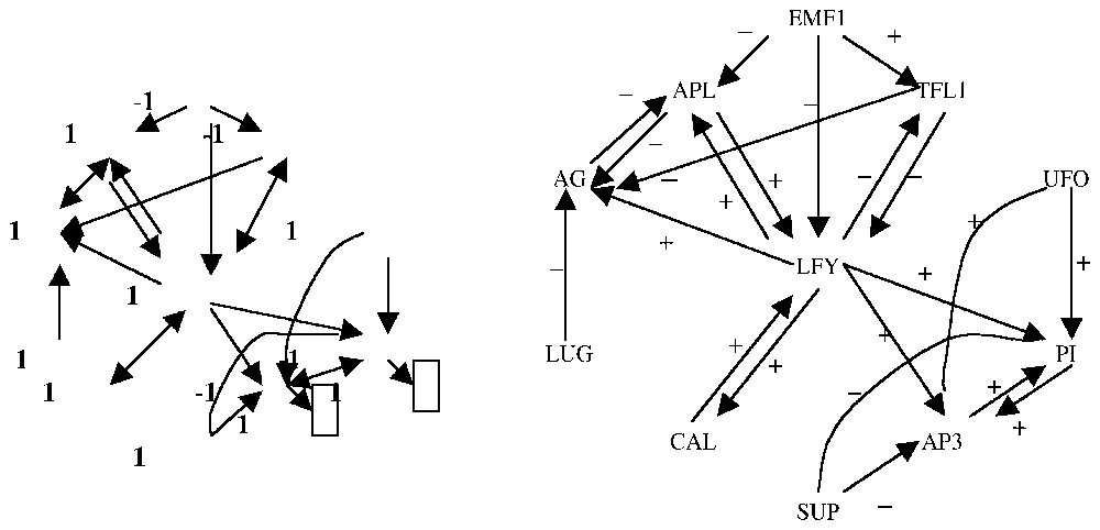
Interaction graph of the flowering genetic regulatory network of Arabidopsis thaliana (right) and an attractor of its Boolean dynamics (left).
For each operon, we can define an interaction matrix , which just expresses that if its coefficient mij is positive (resp. negative), the gene j is a promoter or activator (resp. repressor or inhibitor) of the gene i. If mij is null, then the gene Gj has no influence on the expression of the gene Gi. The interaction graph can be built from the interaction matrix by drawing an edge + (resp. −) between the vertices representing the genes j and i, if mij>0 (resp.<0). In order to calculate the mijs, we can either determine the s-directional correlation ρij(s) between the state vector of gene j at time t−s and the state vector of gene i at times t,t varying during the cell cycle C, or identify the system with a Boolean neural network.
We define the connectivity of the interaction matrix by the ratio between the numbers m of edges of the interaction graph and n of vertices: in general, for known operons and genetic regulatory networks (lactose operon [5,6], Cro operon of the phage λ, lysogenic/lytic operon [4,7] of the phage infecting E. coli, gastrulation regulatory network...), is between 1.5 and 3. The observed induction proportion (number of positive edges divided by m) is between 1/3 and 1/2. If mijs are unknown, we can take them randomly by respecting connectivity and induction proportion.
4 Genetic networks dynamics
If we consider the interaction graph of the flowering genetic regulatory network of Arabidopsis thaliana (Fig. 7) [3], then we can easily define from it a Boolean dynamics with threshold 0: the gene i has the state 1 if it is expressed and −1 if not. The change of state of gene i between the times t and t+1 obeys a majority rule, i.e. we calculate the numbers of its neighbours in state 1 with positive interaction and with negative interaction: if these two numbers are equal, then the new state of i is 1; if the activatory (resp. inhibitory) neighbours dominate, then the new state of i is 1 (resp. −1). When the time t is increasing, the configuration of gene states reaches a stable set of configuration (either a fixed configuration or a cycle of configurations), called an attractor of the genetic network dynamics. In Fig. 7 (left), an example of such an attractor is given, with final states (in black boxes) different from the initial conditions.
We will present now first some qualitative results from the human genome observation, and after some theoretical corresponding statements recently proved:
- – in 1949, Delbrück [17] conjectured that the presence of positive loops (i.e. paths from a gene i to itself having an even number of inhibitions [11]) in the interaction graph was a necessary condition for the cell differentiation; this conjecture has been more precisely written in a good mathematical context by Thomas in 1980 [16];
- – in 1993, Kauffman [22] conjectured that the mean number of attractors for a Boolean genetic network with n genes and with connectivity 2, was equal to √n. This conjecture is supported by real observations: we have about 30 000 genes in the human genome and about 200 different tissues, which can be considered as different attractors of the same dynamics. For Arabidopsis thaliana, and there is 4≈√11 different tissues (sepals, petals, stamens, carpels) [3] and for Cro operon [18] of phage and there is 2≈√5 observed (lytic and lysogenic) attractors.
Recently [8–15], these conjectures have been partially proved. If all loops of the interaction graph are positive, then there exists a state vector x=(x1,…,xn) in {−1,1}n, such that x and −x=(−x1,…,−xn) are fixed configurations of the network dynamics.Proposition 1
If all loops of the interaction graph are negative, then there is no fixed configuration.
Proposition 2
Let a network having n genes and n interactions, then a necessary and sufficient condition of existence of a fixed configuration x is the existence of a positive loop and −x is also fixed.
Proposition 3
Given a state vector , the set of minimal matrices having as fixed configuration is given by the following conditions:Proposition 4
If m is the total number of positive loops C, then the number of fixed configurations is less than or equal to 2m, and this upper bound is reached, if and only if for any positive loop C, there is no edge (x,y)∣x∉C, y∈C.
Proposition 5
If the genetic network has n genes and 2n interactions, then the expectation of the number of its fixed configurations is √n, if n is sufficiently large [15].Proposition 6
If the interaction graph G is a connected digraph without loops having n genes and let suppose that, for any i,bi > 0 and all mijs are positive and verify either (∑jmij⩾bi and, for any k, ∑j≠kmij<bi)=AND rule, or (for each j, mij⩾bi)=OR rule, then the number of fixed configurations is 2(n−1)/2 for n odd, and 2(n−2)/2+1 for n even [14].Proposition 7
Numerous applications of the results above are possible in various regulatory systems [23–40], but we will focus here in the following on a very simple operon governing the choice between the lytic and lysogenic stationary states for Escherichia coli infected by the bacteriophage Mu.
5 An example of operon: the lytic/lysogenic operon of the bacteriophage Mu
Understanding the behaviour of the tempered bacteriophage Mu, considered as a transposon, constitutes a real progress in the knowledge of transposition mechanisms [41].
A Boolean model of the interactions between the expression products of the Mu genome shows the necessity for the removal of the auto-inhibition of the protein Ner (negative loop), which allows the constitutive expression of the phage promoter Pe (positive loop) to demonstrate a bi-stability [11,42]. The presence of the prophage state instability is necessary for the induction of prophages. A review of Escherichia coli factors influencing the Mu behaviour allowed us to propose the Integration Host Factor (IHF) and the Inversion Stimulating Factor (ISF) as being responsible for the removal of auto-inhibition and for the prophagic state instability. The modelling of their effects by a differential system clearly shows the same lytic/lysogenic proportions than those experimentally obtained during the exponential bacterial growth phase and the stationary bacterial growth phase.
These encouraging results demonstrate the necessity of quantitative measures for lytic/lysogenic proportions and intra-cellular concentrations of different Escherichia coli factors during the entire length of the growth cycle, in order to better understand the induction context of the bacteriophage Mu.
The bacteriophage Mu has been discovered in 1963 by L. Taylor [43]. During the infection step, Mu incorporates its DNA and proteins at random locations in the host bacterial chromosome [44]. That induces mutations and new auxotrophies and Mu belongs to the large family of transposable elements [45]. There is two developmental cycles for Mu: after integration in the bacterial chromosome, the Mu DNA is multiplied by a series of replicative transpositions, giving between 50 and 100 new viruses after lysis of the bacterial host (lytic cycle). A weak proportion of infected bacteria becomes lysogenic, the Mu DNA remaining inactive (lysogenic cycle). The induction rate represents the proportion of such lysogenic bacteria entering in the lytic cycle.
Mu infects enterobacteria and in particular E. coli [46] and the integration of its genome into the chromosome of these bacteria involves the phagic transposase pA and its activator pB [47] (cf. Fig. 8). In general, this integrated DNA is amplified through a series of replicative transpositions [48] (involving the transposase pA and its activator pB), then the late phagic functions are synthesized, leading to assembling numerous viral particles dispatched in the extra-cellular medium after the lysis of the host cell. Among a population of infected bacteria, a small proportion will give birth to lysogenic cells, in which the phagic DNA remains passive; this DNA can be replicated during the further mitoses of the lysogenic cell or can enter in a lytic cycle. After integration, the choice between the two possible developmental cycles (lytic or lysogenic) is regulated at the levels of transcription and replicative transposition of the Mu genome.
- – Transcriptional regulation. The viral DNA has a size of 37 kb [49] and possesses two promoters Pe and Pc constitutively expressed [50] (Fig. 8A). The early transcript from Pe codes for the transposase pA, for its activator pB and for a protein Mor activating (via the promoter P and the protein C [51,52]) the cascade of the late functions of the lytic cycle. The transcript coming from Pc codes for the repressor c preferentially fixed on the operators O1 and O2 (Fig. 8B) for repressing Pe and stabilizing the Mu DNA in its inactive form (the prophage DNA). At high concentration, c is also fixed on O3, repressing Pc and hence regulating its own synthesis [53]. The Ner protein is fixed between Pe and Pc and inhibits the transcription from these two promoters [47,54].
- – Transpositional regulation. During the transposition, the transposase pA transiently fix the extremities of the Mu DNA, attL and attR, and the operators O1 and O2 in stabilizing a tetrameric structure, which leads the Mu DNA to a specific configuration, the transposome. The repressor c binds also the extremities of the Mu DNA with a weak affinity [55], entering in competition with pA and then impeaching it to bind the two operators and the two extremities [56]. Hence repressor c inhibits the lytic cycle both at the transcriptional and transpositional levels, and the transposase pA being physically and functionally unstable in vivo [57], the viral genome amplification implies a non-transient expression of the promoter Pe.
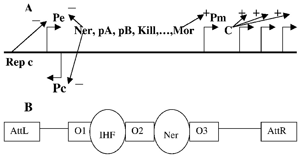
Simplified scheme for the viral DNA of Mu; (A) shows different genes in transcriptional units and the actions of their expression products on the promoters' activity. The fixation sites of the different phagic (e.g., Ner on O2) or bacterial (e.g., IHF on O1) proteic factors are represented in (B).
5.1 Discrete logical (Boolean) model
Experiments about the phage Mu are done during the exponential growth phase of the bacteria for increasing the homogeneity of the observed bacterial states. The lysogenic frequency is highly depending on the used protocol (1% to 50%). We will base our model on lysogenic induction rates observed in exponential phase (0.001%) and in stationary phase (about 100%) (cts 62, temperature 30 °C). For interpreting these experimental data, we used first Thomas' logical approach [16,18,20,21], in which x represents the repressor c and the entity y denotes the group of proteins Pe, Ner, pA, pB, Kill and Mor; their interactions can be designed as in Fig. 9.
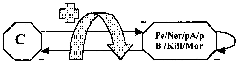
Simplified scheme of the bacteriophage Mu operon (the blue arrow symbolizes the presence of a positive loop).
Variables x and y take values 1 (expression/presence in the cell) or 0 (non-expression/absence from the cell). With this notation, the state Ex, x=1 and y=0 corresponds to the lysogenic state and the state Ey, x=0 and y=1 to the lytic cycle. Let us notice that it is not necessary to explicitly represent the auto-inhibition of the repressor c, because c inhibits Pe and auto-inhibits itself at high concentrations, hence maintaining its concentration between two thresholds θ1 and θ2:
Because the two promoters Pe and Pc are constitutively expressed, x takes the value 1 if it is not inhibited by y: if y=0, then x=1 and if y=1, then x=0. Reciprocally, if x=0, y=1 and if x=1, y=0, leading to the following logic equations:
We consider the four possible initial states Ex (x=1, y=0), Ey (x=0, y=1), Ez (x=0, y=0) and Et (x=1, y=1); if two variables ‘enlightened’ tend to become ‘off’ (noted 1−) or conversely if two variables ‘off’ tend to become ‘on’ (noted 0+), they are not changing at the same time. For example, 0+0+ gives 10 or 01. The behaviour of this system (cf. Fig. 10A) has only a stable stationary state (sss) Ex (x=1, y=0), which corresponds to the lysogenic state. But Mu is a bi-stable system and we have to put another information in the model to get a second sss.
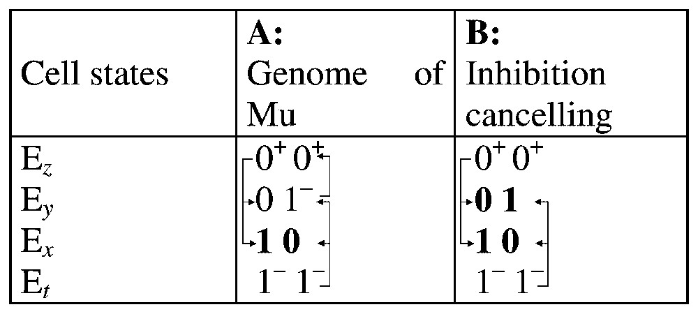
Dynamical behaviour of Mu alone (A) and with a factor cancelling auto-inhibition of y (B). The stationary steady states are represented in bold and superscripts are corresponding to state changes.
For rendering stable the lytic state Ey (x=0, y=1), we need an activation of y cancelling its self-inhibition proportionally to its concentration [11]. In stationary phase, the proportion of lysogenes is near 100%, despite the fact that c is still present. Then we need two factors participating either to the maintenance of the passive phage state, or to the lytic cycle induction (both at the transcriptional and transpositional levels). A review of such possible cellular factors leads to the following list.
- – IHF (Integration Host Factor). IHF is a histone which presents a high affinity for the operator part of the Mu DNA (Fig. 8B), increasing its curvature, hence facilitating the fixation of the repressor c on the operators [58,59] and activating the transcription from the promoter Pe passing over the retro-inhibition by Ner, if c is absent [60]. The absence of IHF impeaches any significative production of phage Mu [61]. The cell concentration of IHF is inversely proportional to the mitosis rate (from 12 000 mol/cell in exponential phase to 52 000 mol/cell in stationary phase [61]).
- – HU (Histone U). It causes the same effects than IHF on transcription and transposition [62], but its concentration does not vary following the bacterial growth rate [61].
- – ISF (Inversion Stimulating Factor). ISF helps c in repressing the lytic cycle: it increases the transcriptional repression and inhibits the transposition [63]; its absence multiplies by about 600 until 800 times the viral particles production in vivo [64]. Cell concentration of ISF is maximal at the start of the exponential growth phase (80 000 mol/cell) and decreases until a rate zero when the growth diminishes [65,66].
- – 8-proteins system. For its DNA replication Mu depends also on host enzymes, from which eight have been identified [67] and for the degradation of the transposase pA and catabolism of c on 2 proteases [41].
5.2 Continuous differential model
IHF is the only bacterial factor activating the transcription of Pe in absence of c. For 01 (Ey) being a stable stationary state (sss), the activation of Pe by IHF has to equilibrate the repression by Ner, leaving the constitutive expression of Pe to run. In stationary growth phase, the induction of prophages is total, despite the presence of a measurable activity of c. The factor ISF helping the action of the repressor c, present in exponential phase but absent in stationary phase, is responsible for that behaviour. Let us now consider a continuous differential model, where the variables are the four states previously considered (Ex, Ey, Et and Ez), IHF and ISF being parameters whose value changes can favour the passage from a state where one of these variables dominates to another state where it is another dominating. The differential system can be written as:
5.3 Results
We have simulated (Mapple Runge–Kutta 4 with constant steps) the dynamical behaviour of 100 000 phages Mu initially in lysogenic state (Ex(0)=105, and Ey(0)=Ez(0)=Et(0)=0), in exponential growth phase ( mol/cell, mol/cell) and in stationary growth phase ( mol/cell, ISF=1 mol/cell) with parameters values equal to k1=100, k2=700, k3=1800, k4=300.
In stationary phase (Fig. 11), the lytic state (Ey) is increasing and reaching a plateau of 100 000 lytic cells, which well corresponds to the experimental data and give an estimation of the duration of the time unit (0.004∼10 days).
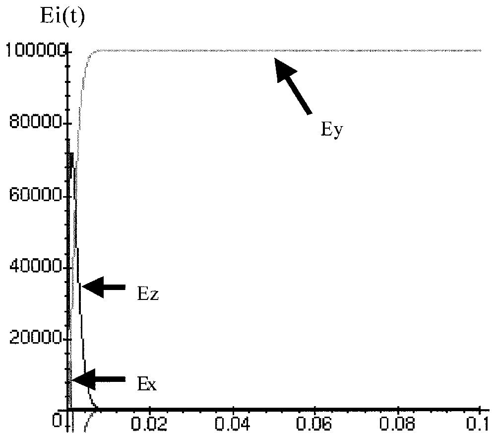
Simulation of the behaviour of 100 000 Mu lysogenes when bacteria are in stationary phase.
In exponential phase (Fig. 12) the lysogenic state (Ex) is practically constant with only a loss of 155 bacteria after 200 days.
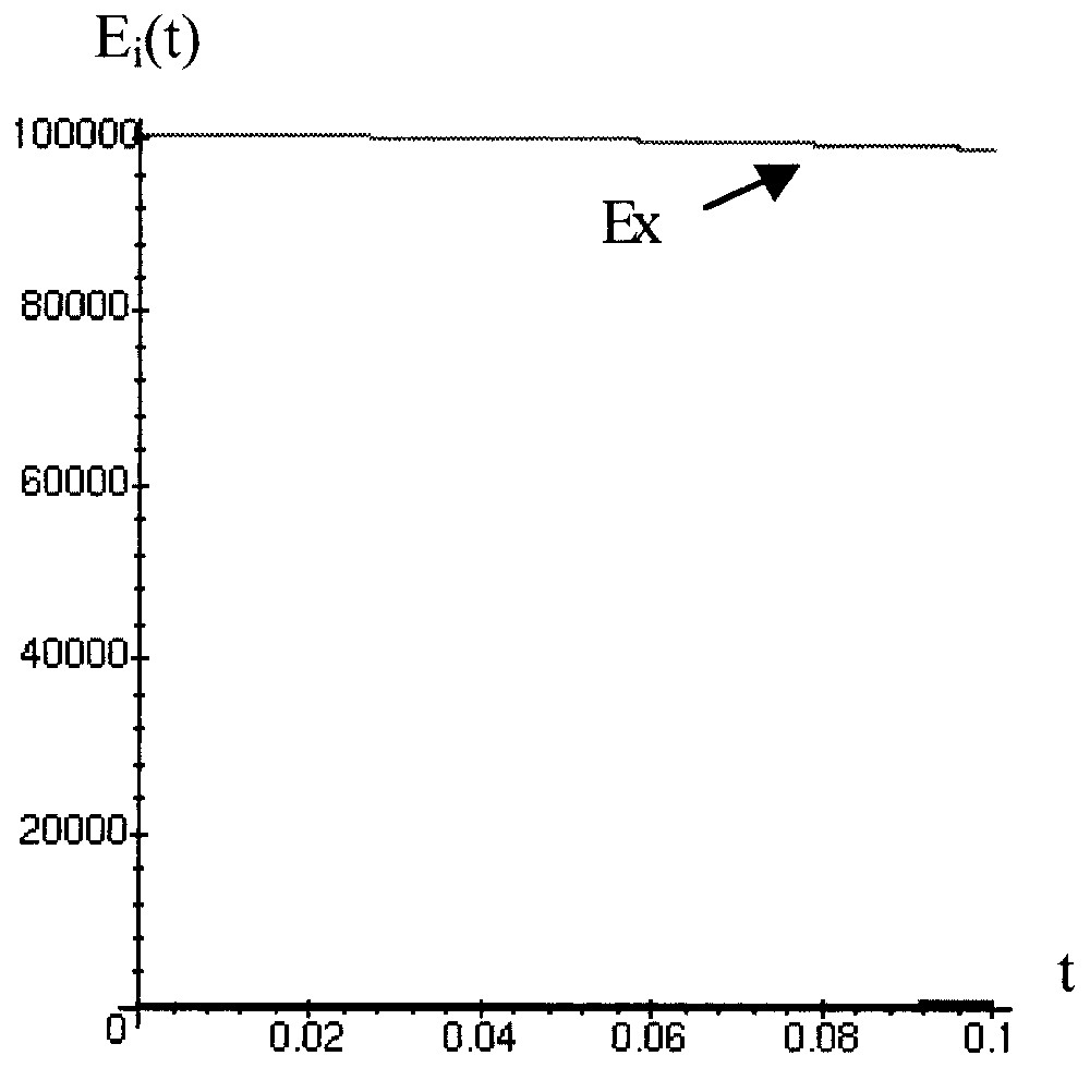
Simulation of the behaviour of 100 000 Mu lysogenes when bacteria are in exponential phase.
To estimate the robustness of these dynamical behaviours with respect to the values of the k1 and k4 parameters, we show that in exponential phase k4 has no incidence and k1 can vary between 10 and 5000 (Fig. 13), without changing the agreement between predicted and observed dynamical behaviours.
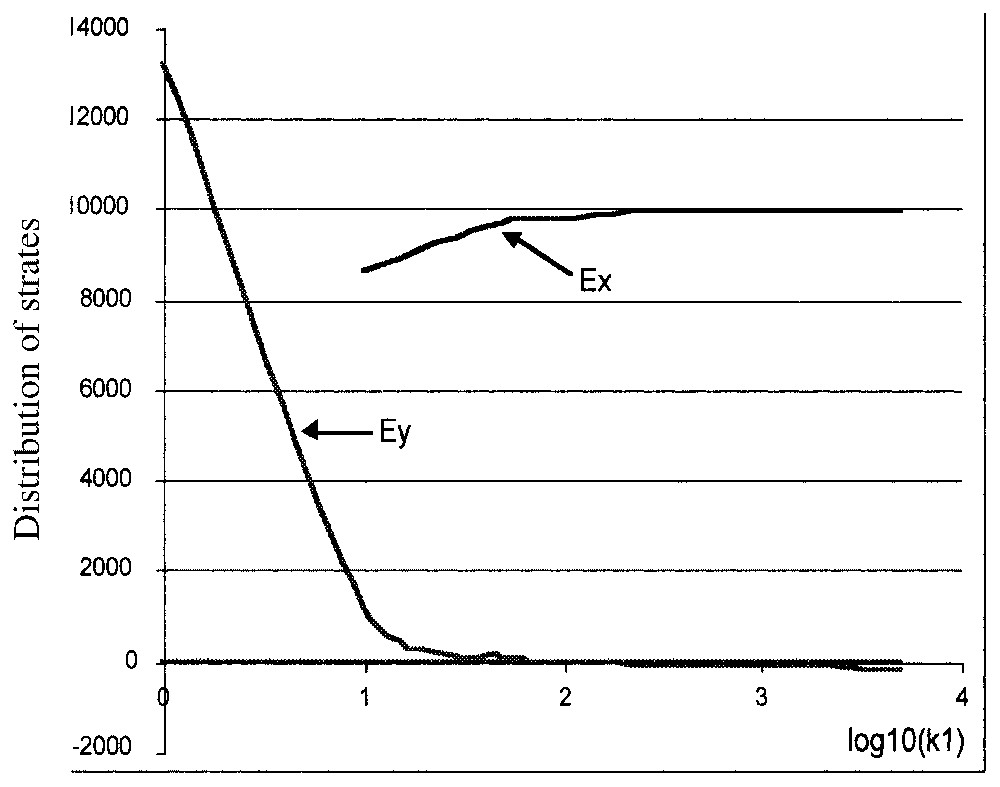
Evolution of the asymptotic values of Ex and Ey in the exponential phase with respect to the k1 values.
The stability study in the neighbourhood of the stationary states is done by calculating the eigenvalues of the Jacobian matrix of the differential system above: 0 is always an eigenvalue that causes an asymptotic instability (but the system is trajectorially Lyapunov-stable) and, in stationary phase, among all other eigenvalues, two are complex, with negative real part, whereas one is real negative; in exponential phase, two are real negative and one is real positive.
5.4 Discussion
The Boolean model has shown the necessity to suppress the self-inhibition by Ner in order to get a bi-stability. The continuous version explains in the lytic phase the reaching a plateau behaviour for the 01 state after 10 days and, in the lysogenic phase, the long transient of the 10 state (1% of decrease after 3 months). In order to get a more predictable model, we need measures of the proportion lytic/lysogenic bacteria on a wider interval of growth rates (the local growth rate R(t) coming from a logistic or from a Monod saturation model [68]). Then the system would become non-linear with ISF and IHF being proportionally respectively to R(t) and dR(t)/dt.
6 Open problems
A frequent criticism made about the Boolean models is their unrealistic number of levels (two); it is possible to easily relax this constraint by considering either a multi-threshold network (for which most of the results of Section 4 are still available), or a non-linear automaton, like the following:
Another perspective exists for the interaction matrices introduced above, i.e. the ability to calculate the barycentre between two matrices by using classical (spectral or L2) distances between matrices, then to build phylogenic trees among a set of species avoiding the complex problems coming from the non-unicity of L1 (Hamming or Manhattan) barycentres met in the sequence based phylogenic trees. The interaction-based phylogenic trees could reflect more the genomic function than the genomic anatomy and hence could explain more deeply the evolution trends, e.g., by distinguishing the evolution of domestic genetic regulatory networks (involved in rearrangements [12,13]) and that of high-level genetic regulatory networks (corresponding for example to brain signalling or hormonal regulatory systems), the complexity of their interaction matrices being probably of the same order of magnitude than the complexity of the metabolic interaction matrices corresponding to their expressed proteins (carriers, receptors or enzymes) [71,72].
A last important open problem concerns the relationship between the number F of fixed configurations and the number S of interaction loops of the interaction matrix : the problem is in fact to find the best upper bound for F given an interaction matrix . This question is the discrete translation of the famous 16th Hilbert's problem of determining an efficient upper bound for the number of limit cycles of a polynomial differential system. Let us summarize the role of the architecture of positive and negative (with an odd number of inhibitions) loops of on the occurrence of multiple stationary behaviours as obtained in [8–15]: if the number of genes and the number of interactions are the same, there is only one isolated loop in and either this loop is negative and the lowest bound (0) for F is reached, or this loop is positive and the upper bound (21) for F is reached. If the numbers of genes and interactions are respectively n and n+1, there are two interaction loops with the following structure; if both loops are negative, F=0; if there are a positive loop and a negative loop disjoint, F=0; if there is a positive loop intersecting a negative loop, F=1; if there are two disjoint positive loops, F=22. If, more generally, the number S of loops is m, then: if all loops are negative, F=0; if all loops are positive, then: 2⩽F⩽2m, and if and only if all loops are positive and disjoint, F=2m. An interesting open problem is now to make exhaustive the determination of F and S and, in particular, to find the circumstances (related to the loops structure) in which we can relate the number of intersecting and isolated loops to F. The approach for solving this open problem could consist first in finding coherent relationships between analogous properties discovered for continuous versions of the regulatory networks and for general Boolean networks.
7 Conclusion
A geneticist could exploit the results given in the above paper as follows: we have shown in Section 4 that it would be possible to characterize the minimal interaction matrices having certain state vectors as fixed configurations. The determination of these matrices is not unique, but permits to focus on certain important equivalence classes, in which the expected matrix has to belong. This considerably restricts the choice of the possible interaction matrices compatible with observed fixed configurations, when it is impossible to directly get from experiments all interaction coefficients, but also when it is only possible to observe the phenomenology of fixed or cyclic configurations. This corresponds in genetics to the phenotypic observation of stationary expression behaviours without experimental measure of the inhibitory and activatory coefficients of promoters and repressors. The possibility to obtain (even in an equivalence class) a sketch of the interaction matrix permits to construct (by randomising the unknown coefficients of ) more complicated interaction matrices, then to test if they still have the observed states as fixed configurations, finally keep or reject these tested matrices and propose further experimental strategies, using bio-arrays for refining the knowledge about the genetic network interaction structure.
Acknowledgements
We have done this work thanks to the support of the National Network for Technology Research RNTS ‘Technologies for Health’ from the French Ministry of Research. We are also indebted to A. Toussaint and C. Ranquet for their helpful discussions concerning the bacteriophage Mu. We thank also B. Hess and A. Winfree (in memoriam) for introducing us to many aspects of the dynamics of life.