Adaptive branching in Evolution and Epigenesis

Yannida L. Kergosien

doi:10.1016/S1631-0691(03)00113-6

Résumés

Anglais
Français

We describe one of the simplest models that exhibit an adaptive branching behaviour. It is analysed both experimentally and formally, and its successive bifurcations provide a good model of what R. Thom called ‘generalized catastrophes’. Two theorems on the stochastic adaptivity of the algorithm to very general shapes of target are given. The model further displays the phenomenon of abortive branching: each macroscopic branching appears after a burst of microscopic branchings that stop growing after a very short time. The mathematical analysis of the model explains why and how this behaviour occurs. Possible applications of these models to Evolution (natural and artificial) and Epigenesis are briefly mentioned, and a higher dimensional version is applied to growing a tree in a space of shapes in the context of a database of medical images.

Nous décrivons un des modèles mathématiques les plus simples qui soit capable de ramification adaptative et étudions sa pertinence biologique. Ayant défini dans un espace une probabilité chargeant une région appelée cible, et un ensemble appelé graine, état initial du réseau à faire croître, chaque tirage d'un point au sein de la cible définit un nouveau point à ajouter au réseau. On peut observer expérimentalement l'apparition d'arborescences qui adaptent progressivement la forme du réseau à celle de la cible. On peut aussi montrer plusieurs théorèmes d'adaptativité stochastique du réseau à des cibles très générales. L'étude plus fine des ramifications révèle l'existence du phénomène de ramifications abortives, dont l'étude formelle s'apparente au concept de catastrophe généralisée. Ce modèle est applicable à l'espace tridimensionnel pour modéliser l'épigénèse, mais aussi à des espaces de dimension plus grande, comme des espaces de formes, dont nous discutons quelques applications dans le cadre de l'évolution en biologie et pour des applications de bases de données de formes en imagerie médicale.

1 Introduction

1.1 The adaptive branching phenomenon in Biology

Branching phenomena are very common in Biology, and often related to some adaptation. They can take place in physical spaces when epigenetic morphogenesis is the question. There they can be compared to or related to the morphological branching phenomena which rivers, sparks, or transportation networks display, where some variational or optimality principle can be recognized. It is tempting to look for some function being optimized as soon as some tree morphology is recognized, starting from plant biology! But one can also think of using trees when the objectives are given by humans and to be met by technology. Algorithmics has been such a fertile field of application. Even in Biology, trees occur in more abstract spaces, like those where phylogenetic trees are constructed. There also, one can either consider these trees as given and try to explain them from simpler principles, or use trees as a tool to explore and understand complex data spaces such as those which arise from the collaborative biological research.

The algorithm we are going to present can be used in both ways. We will study some of its features in a naturalist's way, so as to be able to look for similar patterns in biological phenomena and perhaps infer some interesting properties. On the other hand, its power can be used for more technologically oriented problems like the one we briefly mention at the end of this paper.

1.2 Some other simple models

Looking for the simplest models for adaptive branching, one has first to consider physical phenomena that can exhibit such a behaviour. Among them, diffusion-based models have been studied very early, for instance in relation to crystal growth. Diffusion can be coupled to reaction (after A.M. Turing) or to other phenomena like accretion, and involve a number of diffusible species. The biologically oriented models of Gierer and Meinhard [1] used two diffusible species. In [2,3] we described how to get adaptive branching with a single one, but the interesting range of parameters was limited and the phenomenon rather unstable. In the sequel, we will consider a model less directly relevant to physical epigenesis but very robust and perhaps better adapted to the study of branching in abstract biological spaces. We still view this model as of an epigenetic flavor in that we do not use any ‘preformation’ or genetic information.

2 A simple adaptive branching algorithm

2.1 Definitions, the algorithm

Here we introduce the algorithm in a simple setting, which is not the most general one. The evolution takes place in the usual p-dimensional space $ℝ^{p}$ . A fixed subset of it, finite or not, is called the target and noted C, with a probability defined on it. A second subset of $ℝ^{p}$ , which we call the network, is going to be modified (it will ‘grow’) at each step of the algorithm. We shall note R_n the network after step n. Starting with an initial network R₀, each step will add a point to the network.

To start, one needs to define an initial network R₀, a target C with its probability distribution, and a real number $ϵ \in] 0, 1 [$ . At each step, say i, we:

– randomly draw a point, say a_i, from the target (using the given probability distribution);
– look for b_i, the point of the network R_i−1 which is closest to a_i;
– compute b′_i=ε·a_i+(1−ε)·b_i;
– ‘graft’ b′_i on the set R_i−1 to get R_i=R_i−1∪{b′_i}.

The stopping criterion can be the number of steps, or some condition on the network. The case of a tie for the choice of b_i formally calls for a procedure, either stochastic or deterministic, to choose b_i, but those cases are very unprobable (we will not develop that issue here). The formula to compute b′_i uses vector (or affine) algebra; typically ε is taken small, making b′_i close to b_i but slightly displaced in the direction of a_i.

Since each point added to the network is related to a definite point of the former network, the network has the structure of a finite tree if R₀ was a single point (and a finite set of finite trees in general). Branching points can thus be defined as points with more than one point grafted, besides ‘continuation points’ (points with only one graft) and ‘tip points’ (points with no graft). One could include in the definition of the network the line segments joining points to their grafted sons and compute closest points on this object, but we will not do it.

2.2 Experimental results

Fig. 1 shows the result of the algorithm for a target being a line segment with uniform probability distribution, starting from a single point, and for ε=0.001. The network grows toward the target and branches several times in a way that looks adapted to the geometry of the target.

Fig. 1
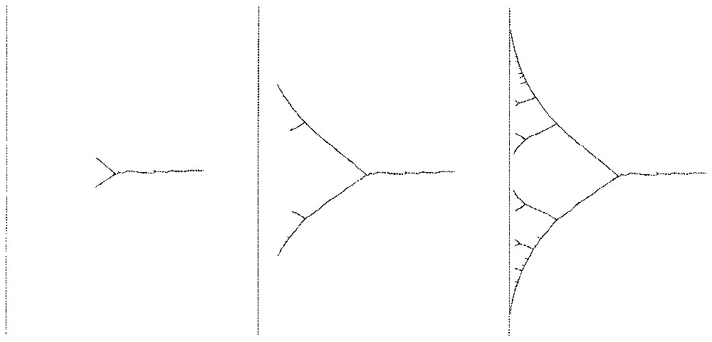
Linear target (left): network after 1000, 5000, 25000 steps.

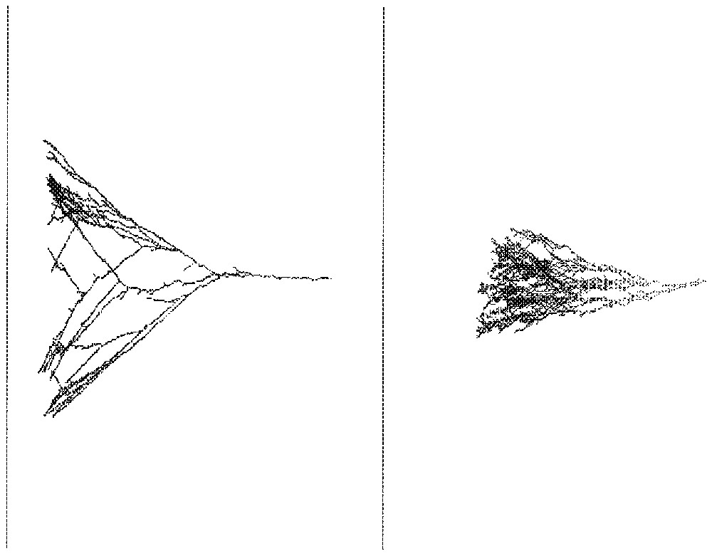
Starting from two points as the initial network can lead either to cooperation in a ‘market sharing’ way or to a ‘winner takes all’ competition, depending on the situation of the two seeds and the geometry of the target (Fig. 2).

Fig. 2
Two seeds either sharing the target (left) or competing for it (right).

Adaptation to more complex shapes of targets is also seen. In Fig. 3, the network adapts to two different targets (i.e. two components of the target) the one on top being a circle with uniform probability and the bottom one being a disk with uniform probability, with the disk getting a total of four times more probability than the circle. On that figure the target has not been drawn. Notice the different morphologies of the network in the two cases.

Fig. 3
Evolution to a target (undrawn) made of a circle (top) and a disk (bottom).

This algorithm can be used in higher dimensional spaces. Fig. 4 shows on the left a network growth from a point seed in $ℝ^{6}$ towards a 5-dimensional hypercube target. What is shown is the projection of the network onto a plane perpendicular to the target and which contains the seed. On the right of Fig. 4, the network is shown growing in $ℝ^{50}$ towards a 49-dimensional hypercube with the same conventions. Superimpositions due to the projection get of course more numerous in that case.

Fig. 4
Growth of a network in $ℝ^{6}$ (left) and in $ℝ^{50}$ (right).

2.3 Adaptivity theorems

The former experimental results are supported by the following two theorems, which show the adaptive power of the algorithm. To state them, we slightly modify our definitions. Instead of defining first the target and then a probability on it, we start with a probability on $ℝ^{p}$ and define the target as the set of points of $ℝ^{p}$ for which any neighbourhood has positive (i.e. >0) probability (this set is known as the support of the probability measure). We shall write B(x,r) for the open ball ${y \in ℝ^{p} ∣ d (x, y) < r}$ , where x is the centre and r is the radius, and d is the Euclidean distance.

The first theorem states that any neighbourhood of the target will be eventually approached by the network as close as we want with a probability as close to 1 as we want. To state it formally, we choose a ball B(x,r) intersecting the target, and a slightly larger concentric ball B(x,r′), together with a probability value 1−η as close to 1 as we wish. We then state that, under these conditions, there is always a definite number of steps after which the probability that some points of the network have entered the larger ball is at least the probability value chosen in advance.

Theorem 1

Let E stand for $ℝ^{p}$ with p⩾2. Then for any $ϵ \in] 0, 1 [$ , for any η>0, for any x∈E, any r>0 such that P[B(x,r)]>0 and any r′>r, there exists a positive integer N such that for any integer n>N, P[B(x,r′)∩R_n≠∅]>1−η, i.e. the probability that some points of R_n are in B(x,r′) is greater than 1−η.

The second theorem states that when the target is bounded, all its points can be simultaneously approached by points of the network as close as we want, with a probability as close to 1 as we want if we wait long enough. More formally, for any distance value r>0 and any probability value 1−ε, there is a definite number of steps after which the property that all the points of the target will be at a distance less than r from the network will hold with a probability greater than 1−ε.

Theorem 2

Assume the target C to be bounded. Then for any ε in $] 0, 1 [$ , for any η>0, for any r>0, there exists a positive integer N such that for any integer n>N, the probability that sup_c∈Cd(c,R_n)<r is greater than 1−η (i.e. the probability that there exists a point c in the target not within a distance r from the network is less than η).

Consequence

Let us define an active point of a network as a point which, for at least one point of the target, is the closest among the network points: it is thus a point which still has a non-zero probability of being grafted. A consequence of the second theorem is that after the same number N of steps, and with the same probability, no active point of the network remains further than r from the network. Thus, whereas the network is an increasing set with a part of it (the active set) approaching the target, the active set really tends to fit the target, leaving no point behind.

3 Abortive branchings

Decreasing ε usually makes branches straighter, and one could think that in the limit the algorithm tends to the clean branchings and smooth branches of a deterministic process. This does not happen, because a particular phenomenon occurs repetitively in the vicinity of macroscopic branchings: many small branchings appear, but are soon inactivated by one of their branches winning over the other one. We called ‘abortive bifurcations’ this phenomenon [3]. Analysing the 2-dimensional case leads to a good understanding of the phenomenon.

3.1 The geometry of branching

Branching occurs when some grafting takes place at a point of the network, say A, which is not a tip. This implies that A is closer to some point of the target than any point on the branch already grafted on A.

3.2 Demonstrating abortive bifurcations

Fig. 5 shows an instance of successive abortive bifurcations before a macroscopic branching appears. To see them, one should use small ε and magnify the network at a distance from the target where a macroscopic branching is likely to occur. Notice the constant qualitative pattern of the network at each abortive bifurcation: after one of the branches wins over the other one, i.e. ‘hides it’ from the target (the winner being closer than the other to any point of the target, the loser cannot grow anymore), the network bends back to the centre of the target. In some contexts like Evolution, such repetition of abortive attempts of differentiation might be looked for and perhaps used to detect the imminence of a major branching.

Fig. 5
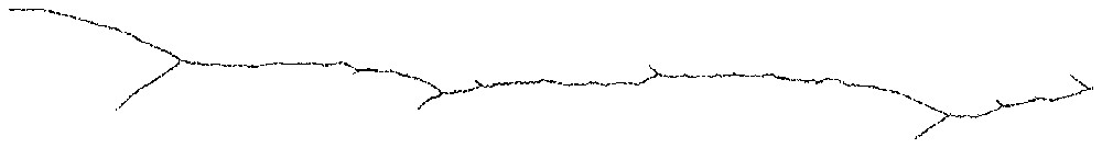
Small abortive bifurcations slightly before a stable branching (going right to left).

3.3 Analysis of abortive branching

To understand why abortive branching happens repetitively before a major branching can remain, one can restrict the study to the simple 2-dimensional case with a linear target. The evolution of the two tips, say X and Y, that arise from a branching can be summarized by the evolution of the vector Y−X. Each of the two tips hides the other one and wins when the vector crosses one of two lines (we call them critical) related to the ends of the target. The evolution of the vector is stochastic, but the expectation of the dynamical system that governs it can be computed easily from the target geometry and the position of the tips. Fig. 6 shows the phase portraits of the dynamical system acting on the vector and the critical lines for two different distances to the target. When far from the target, all the trajectories eventually cross one of the winning lines. Getting closer to the target modifies the picture, and a growing number of trajectories are able to make their way without hitting either of the critical lines, meaning that the branching did not abort. The real vector field that acts on the couple of tips can be viewed as the sum of that deterministic (expected) field and a stochastic component that can be made small with ε small. The whole picture thus involves a bifurcation stochastically perturbed, the deterministic part of which depends on the position relative to the target. It fits with the idea of a ‘generalized catastrophe’ proposed for study by Thom in [4].

Fig. 6
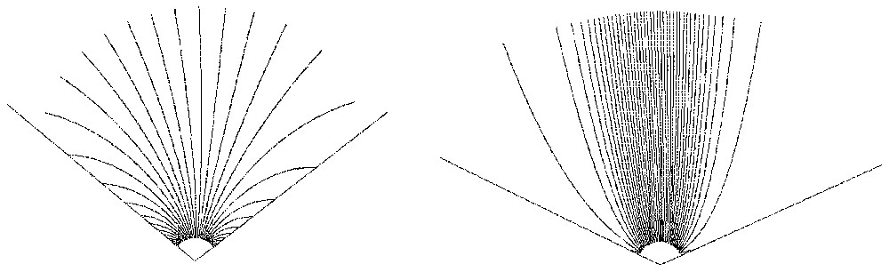
Phase portraits far from (left) and close to (right) target.

4 A modified algorithm

4.1 Some implementation issues

At each step of the algorithm, one has a to find a closest point within the network. But many points may become irreversibly inactive and it is computationally more efficient to periodically detect and mark inactive points to avoid testing them for proximity (one can also maintain a list of active points: several variants and data structures can be used). A network point x gets inactive when the active points y₁,…,y_k of the network collectively ‘hide it’ from all the target points, i.e. when for any target point c there is always a y_i such that d(y_i,c)<d(x,c). Sometimes a simple criterium can find some of the inactive points. For instance, when the target is a line segment with end points c₁ and c₂, for a point x in the network to be inactive, it is enough that there exists another point y in the network such that d(y,c₁)<d(x,c₁) and d(y,c₂)<d(x,c₂). This rule generalizes to polytopes (either for the target or a bounding box for it) and their extreme points in higher dimensions, but such information is not always easy to get in applications. More powerful rules have to adapt to complex target shapes and do not share the simplicity and versatility of the algorithm. Another reason for modifying the algorithm is the number of comparisons to be performed, even if active points have been selected.

4.2 Avoiding garbage collection and using search trees

We experimented with success a modified version of the algorithm, where a binary search tree is used to locate the closest points, and where no garbage collection is needed. The new rule is that after some branching occurs, one definitively assigns a part of the target to the future growth of each of the two branches. After each target point has been drawn, one thus first locates the branch to be grown by successively comparing the distances to couples of sons of the former branchings points, starting from the root (a classical binary search in a tree). Such algorithm remains very efficient even with large trees in high-dimension spaces. It also behaves quite like the former one, with good adaptive properties, but of course with no abortive bifurcations, since the subregions of the targets cannot move after each bifurcation.

5 Growing trees in shape spaces

Discrete trees have extensively been used by search algorithms to organize comparisons. There is also a place for continuous trees to organize morphogenetic or evolutive processes into continuous branching families of shapes. These viewpoints fuse in the technology of databases for continuously varying data like images or 3-dimensional protein shapes. We experimented the former algorithm to grow trees in a space of shapes extracted from medical images, using as the target the set of all the sections of a complex bone (human scapula). The original surface was reconstructed from a set of parallel sections acquired from CT-scanner. Considering any possible section in any direction leads to a very complex family of curves where queries are problematic. Each sectional curve is a set of polygons (some of the sections are not connected) but so far we kept only a single component so as to be able to use a simple matching procedure. Randomly drawing sections from a set of 962 possible sections, and starting from a simple shape like a circle (approximated by a 100-sided polygon), we could grow a tree in the shape space and observe branchings that progressively led to the actual members of the set of sections. When searching for closest curves, prior matching was used, in order to focus on shape, before computing the element to be added to the network using an interpolation between each new target curve and the closest network curve. Fig. 7 shows the inner nodes of the tree thus obtained (grown from right to left, after 500 steps, with ε=0.09, for a computing time of 35 seconds on a 500-MHz Pentium processor). Observe the progressive differentiation of shapes towards different morphologies in the target space. Once grown, the tree can be used for fast retrieval and classification of an unknown sectional curve [5], comparing it first with the root's section, then with right and left children at each branching, like with binary search trees. Such methodology could be compared to some of the procedures used in exploratory statistics [6], but here we emphasize the construction of a continuous family with branchings that could be used in the comparison and study of complex biological objects. Also our first algorithm can be compared to Kohonen's self organizing maps [7] despite different behaviour.

Fig. 7
Inner nodes of a tree grown in the space of shapes of plane sections of a human scapula (right to left).

6 Conclusion

A simple stochastic algorithm has been described, which can adapt a finite subset with a tree structure to very general targets in $ℝ^{p}$ . A major advantage of it is the small number of parameters to be chosen and the robustness of the adaptivity property. The adaptivity properties have been illustrated experimentally and supported by two theorems. The phenomenon of abortive bifurcations has been analysed and its pertinence to problems in biological evolution has been briefly mentioned. As an application to databases of shapes, a tree is grown in a space of curves taken from medical images.

Appendix A Proofs of the adaptivity theorems

We want to prove that $\forall ϵ \in] 0, 1 [$ , ∀η>0, ∀x∈E, ∀r>0 such that P[B(x,r)]>0, ∀r′>r, $\exists N \in ℕ$ : ∀n>N, P[B(x,r′)∩R_n≠∅]>1−η where R_n is the network after the nth accretion. A problem is that successive accretions due to points drawn from B(x,r) may grow different branches of the network instead of adding their effects to the same tip. We thus choose a ball B(y,ξ)⊂B(x,r) with P[B(y,ξ)]>0, where ξ is a positive real number small enough (to be computed later). We know from elementary probability results that waiting long enough guarantees us to witness as many drawings from B(y,ξ) as we wish, whatever the smallness of P[B(y,ξ)]. We will call a₁,… the points drawn from B(y,ξ), b₁,… the corresponding closest network points, and b′₁,… the points consequently added to the network. We call b₀ the point of the initial network R₀ closest to B(y,ξ), and l_i=d(a_i,b′_i). If we can get a b′_i close enough to its a_i, it has to be in B(x,r′) and we are done. Let us compute how l_i decreases with i:

l_{i + 1} = d (a_{i + 1}, b'_{i + 1}) = (1 - ϵ) d (a_{i + 1}, b_{i + 1}) ⩽ (1 - ϵ) d (a_{i + 1}, b'_{i})

(since otherwise b_i+1 would not be closer to a_i+1 than b′_i)

⩽ (1 - ϵ) (d (a_{i + 1}, a_{i}) + d (a_{i}, b'_{i})) ⩽ (1 - ϵ) (2 ξ + l_{i})

If we took ξ such that, for all the l_i we need,

ξ ⩽ \frac{ϵ l_{i}}{4 (1 - ϵ)}

then

l_{i + 1} ⩽ (1 - ϵ / 2) l_{i} ⩽ {(1 - ϵ / 2)}^{i + 1} l_{0}

Just choose k big enough to get

l_{k} ⩽ {(1 - ϵ / 2)}^{k} l_{0} < r' - r

and take ξ accordingly. After k points have been drawn from the B(y,ξ) you chose, which happens with a probability greater than 1−η after a computable number N of steps of the algorithm, the network will have entered B(x,r′).

The second theorem states that $\forall ϵ \in] 0, 1 [$ , ∀η>0, ∀r>0, $\exists N \in ℕ$ such that ∀n>N, P[sup_c∈Cd(c,R_n)<r]>1−η. Cover C with balls of radius r/3. Using the compacity of C (which is always closed, and bounded by hypothesis), extract a finite covering (B(c_i,r/3))_1⩽i⩽M. Apply the former theorem and a simultaneous inference argument to get N such that with a probability greater than 1−η:

\forall 1 ⩽ i ⩽ M \exists b_{j} \in R_{n} : b_{j} \in B (c_{i}, 2 r / 3)

Then with probability greater than 1−η:

\forall c \in C \exists j, 1 ⩽ j ⩽ M :

d (c, R_{n}) ⩽ d (c, c_{j}) + d (c_{j}, b_{j}) < r / 3 + 2 r / 3 = r

The consequence on the active set is obvious: if any point of the target is less than a distance r away from the network, then no point of the network can be active unless it is within that distance from the target.