Liénard systems and potential–Hamiltonian decomposition – Applications in biology

Loïc Forest; Nicolas Glade; Jacques Demongeot

doi:10.1016/j.crvi.2006.12.001

Biological modelling / Biomodélisation

Liénard systems and potential–Hamiltonian decomposition – Applications in biology
[Systèmes de Liénard et décomposition potentielle–hamiltonienne – Applications en biologie]

Présenté par : Michel Thellier

Loïc Forest ¹ ; Nicolas Glade ¹ ; Jacques Demongeot ^1,²

¹ TIMC – IMAG, UMR CNRS 5525, université Joseph-Fourier, Grenoble, faculté de médecine, 38700 La Tronche, France
² Institut universitaire de France

Comptes Rendus. Biologies, Volume 330 (2007) no. 2, pp. 97-106.

Résumés

Anglais
Français

In separated notes, we described the mathematical aspects of the potential–Hamiltonian (PH) decomposition, in particular, for n-switches and Liénard systems [J. Demongeot, N. Glade, L. Forest, Liénard systems and potential–Hamiltonian decomposition – I. Methodology, II. Algorithm and III. Applications, C. R. Acad. Sci., Paris, Ser. I, in press]. In the present note, we give some examples of biological regulatory systems susceptible to be decomposed. We show that they can be modelled in terms of 2D ordinary differential equations belonging to n-switches and Liénard system families [O. Cinquin, J. Demongeot, High-dimensional switches and the modeling of cellular differentiation, J. Theor. Biol. 233 (2005) 391–411]. Although simplified, these models can be decomposed into a set of equations combining a potential and a Hamiltonian part. We discuss about the advantage of such a PH-decomposition for understanding the mechanisms involved in their regulatory abilities. We suggest a generalized algorithm to deal with differential systems having a second part of rational-fraction type (frequently used in metabolic systems). Finally, we comment what can be interpreted as a precise signification in biological systems from the dynamical behaviours of both the potential and Hamiltonian parts.

Dans des notes séparées [J. Demongeot, N. Glade, L. Forest, Liénard systems and potential–Hamiltonian decomposition – I. Methodology, II. Algorithm and III. Applications, C. R. Acad. Sci., Paris, Ser. I, in press], nous avons décrit la décomposition potentielle–hamiltonienne pour des systèmes de type n-switch ou de Liénard. Leurs équations sont bien adaptées à la modélisation des systèmes dynamiques en biologie. Nous donnons ici des exemples de systèmes de régulation biologique pouvant être écrits sous la forme d'équations de Liénard et également sous forme de systèmes n-switch [O. Cinquin, J. Demongeot, High-dimensional switches and the modeling of cellular differentiation, J. Theor. Biol. 233 (2005) 391–411]. Nous discutons ensuite de l'intérêt de connaître les contributions potentielles et hamiltoniennes de ces systèmes pour la compréhension de leurs mécanismes. Pour terminer, nous suggérons un algorithme prenant en compte des systèmes différentiels à second membre de type fraction rationnelle rencontrés dans les modèles métaboliques, pour lesquels les parties potentielle et hamiltonienne ont des significations biologiques précises. On explique comment utiliser en pratique cette décomposition au voisinage de leurs attracteurs.

Métadonnées

Reçu le : 2006-11-28
Accepté le : 2006-12-05
Publié le : 2007-01-16

PMID

DOI : 10.1016/j.crvi.2006.12.001

Keywords: Liénard systems, Potential–Hamiltonian decomposition, Dynamical systems, Regulatory systems, n-Switches, Metabolic systems, Periodic biological systems, Systems biology
Mot clés : Systèmes de Liénard, Décomposition potentielle–hamiltonienne, Systèmes dynamiques, Systèmes de régulation, n-Switchs, Systèmes métaboliques, Systèmes biologiques périodiques, Biologie des systèmes

Affiliations des auteurs :

Loïc Forest ¹ ; Nicolas Glade ¹ ; Jacques Demongeot ^{1, 2}

¹ TIMC – IMAG, UMR CNRS 5525, université Joseph-Fourier, Grenoble, faculté de médecine, 38700 La Tronche, France
² Institut universitaire de France

@article{CRBIOL_2007__330_2_97_0,
     author = {Lo{\"\i}c Forest and Nicolas Glade and Jacques Demongeot},
     title = {Li\'enard systems and {potential{\textendash}Hamiltonian} decomposition {\textendash} {Applications} in biology},
     journal = {Comptes Rendus. Biologies},
     pages = {97--106},
     publisher = {Elsevier},
     volume = {330},
     number = {2},
     year = {2007},
     doi = {10.1016/j.crvi.2006.12.001},
     language = {en},
}

TY  - JOUR
AU  - Loïc Forest
AU  - Nicolas Glade
AU  - Jacques Demongeot
TI  - Liénard systems and potential–Hamiltonian decomposition – Applications in biology
JO  - Comptes Rendus. Biologies
PY  - 2007
SP  - 97
EP  - 106
VL  - 330
IS  - 2
PB  - Elsevier
DO  - 10.1016/j.crvi.2006.12.001
LA  - en
ID  - CRBIOL_2007__330_2_97_0
ER  -

%0 Journal Article
%A Loïc Forest
%A Nicolas Glade
%A Jacques Demongeot
%T Liénard systems and potential–Hamiltonian decomposition – Applications in biology
%J Comptes Rendus. Biologies
%D 2007
%P 97-106
%V 330
%N 2
%I Elsevier
%R 10.1016/j.crvi.2006.12.001
%G en
%F CRBIOL_2007__330_2_97_0

Loïc Forest; Nicolas Glade; Jacques Demongeot. Liénard systems and potential–Hamiltonian decomposition – Applications in biology. Comptes Rendus. Biologies, Volume 330 (2007) no. 2, pp. 97-106. doi : 10.1016/j.crvi.2006.12.001. https://comptes-rendus.academie-sciences.fr/biologies/articles/10.1016/j.crvi.2006.12.001/

Version originale du texte intégral

1 Introduction

Liénard and n-switches systems have served as paradigm or toy models for many biological regulatory systems (cardiac, respiratory, neural...) and morphogenetic processes (e.g., in embryogenesis and neogenesis), presenting a periodic temporal behaviour with relaxation waves for excitable cells isolated or connected in functional tissues and spatio-temporal patterns if they belong to regulatory and/or morphogenetic networks. In tissues, these interacting cells can cause solitary waves or periodic spatial structures stationary in time (participating to the determination of the anatomy of the tissue by generating the morphology of the corresponding organ). They can also produce periodic structures in time, acting as intercellular or tissular signal triggers, e.g., provoking a collective behavior, the best example being the cardiac tissue in the heart. These systems are frequently used. We give here some examples of their use.

2 The n-switches as morphogenetic models

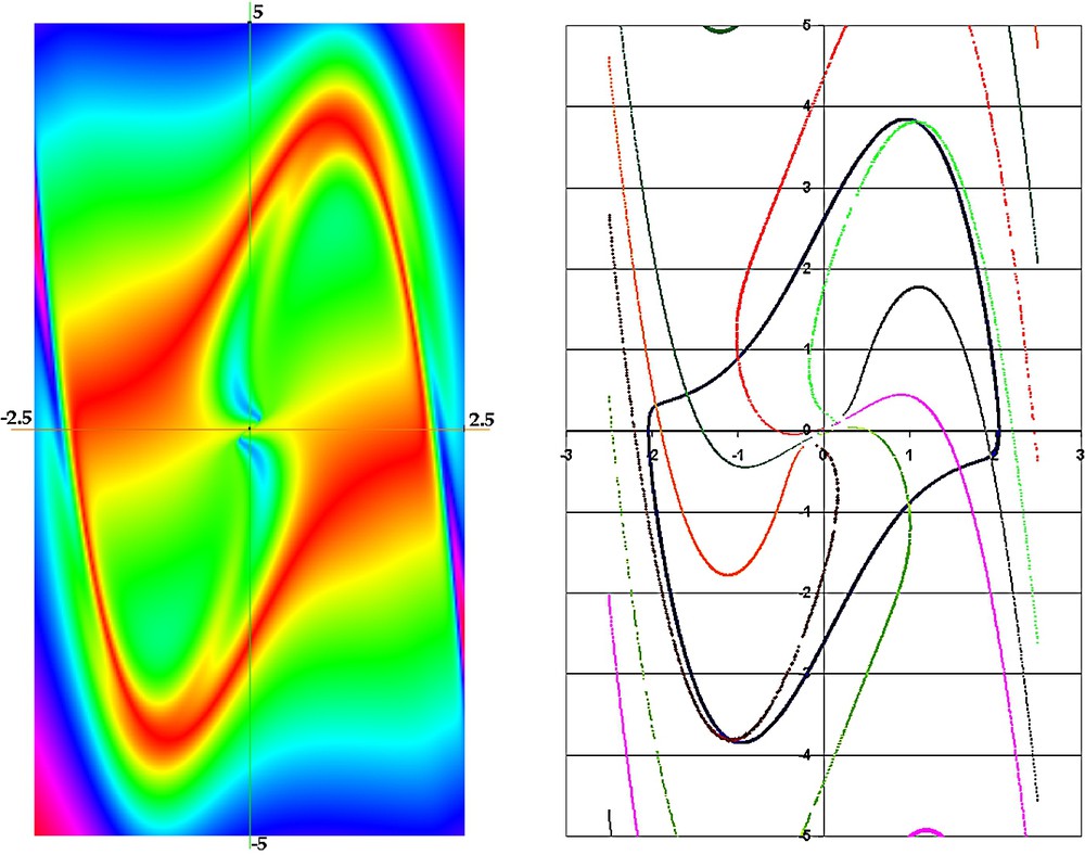
n-Switches have been proposed in [2] and can be used to model neural [3] or metabolic networks [4–10] based on the existence of inhibitory mediators, proteins or hormones like those encountered in the functioning and embryogenesis of the neural system or in plant morphogenesis. In [3], in the neural case, it is noticed that “it is easy to see that in these networks each neuron inhibits all the others; consequently if one starts firing, it keeps the rest silent”. The mathematical properties of n-switches have been already studied in [2], in particular, their ability to be represented by a pure potential system. We give in Fig. 1 (left) an example of 2D patterns obtained for a 3-switch implemented through a cellular automaton in which a cell i is surrounded by cells j's, belonging to a neighbourhood $V (i)$ , in which we fixed the weights $w_{i j}$ in agreement with Table 1, where the central cell i has the maximum weight $w_{i i}$ and the peripheral cells j's the minimum weights $w_{i j}$ .Then the automaton transition is defined by:

Fig. 1
(Left) Approximation of 2D morphogenetic frontiers in a 3-switches automaton, with (A) initial condition and (B) (resp., (C)) near the asymptotic behavior for an opposite (resp. inserted) red region. The blue regions correspond to cells that have not yet reached their asymptotic state. (Right) (D) Algebraic approximation of a route to the chaos for a 3D Lotka–Volterra system.

1 (cell $j_{1}$ )	1	1	1	1
1	2	2	2	1
1	2	4 (cell i)	2	1
1	2	2	2	1
1	1	1	1	1 (cell $j_{24}$ )

(i) $x_{i} (t)$ denotes the state (whose value e is $black = 0$ , $green = 1$ , $red = 2$ ) of cell i at time t; an indicator variable $y_{i}$ is defined by:
$y_{i} (e, t) = {\begin{matrix} 1 & if x_{i} (t) = e \\ 0 & if not \end{matrix}$
(ii) $A (e, i) (t)$ is the age of the cell i in state e at time t (i.e., the number of previous consecutive iterations where cell i was in state e before reaching the state $x_{i} (t) = e$ at time t).
(iii) Thresholds for a cell i at time t are denoted by $s_{k} (e, i) (t)$ and are calculated from basic values $s_{0}$ , $s_{1}$ and $s_{2}$ and from aging parameters $ν_{1}$ and $ν_{2}$ (in the following, $ν_{1} = ν_{2} = 1 / 2$ ):
$if x_{i} (t) = 2, s_{2} (2, i) (t) = s_{2} - A (2, i) (t) v_{2} s_{2} (1, i) (t) = s_{1} + A (2, i) (t) v_{2} s_{2} (0, i) (t) = s_{0}$
$if x_{i} (t) = 1, s_{1} (2, i) (t) = s_{2} + A (1, i) (t) v_{1} s_{1} (1, i) (t) = s_{1} - A (1, i) (t) v_{1} s_{1} (0, i) (t) = s_{0}$
$if x_{i} (t) = 0, s_{0} (2, i) (t) = s_{2}, s_{0} (1, i) (t) = s_{1} s_{0} (0, i) (t) = s_{0}$
(iv) if $x_{i} (t) = e$ , $x_{i} (t + 1) = f$ ,
$if p = \sum_{j \in V (i)} w_{ij} y_{j} (f, t) / \sum_{j \in V (i)} w_{ij} ⩾ s_{e} (f, i) (t) .$
If several thresholds are reached, we choose the state f with the probability p.

The above condition (iv) expresses the fact that i is taking the state f at time $t + 1$ if there are enough cells j's in its neighbourhood $V (i)$ in this state f at time t. The inequality in (iv) is qualitatively analogous to the competitive inhibition equation of a 3-switch [2]. Fig. 1 (left) exhibits two asymptotic behaviours showing the possibility of both two morphological regions in opposition (B) and one region inserted (C). It could be interesting now to exhibit, as for the original n-switch system [2], a potential function driving its asymptotic evolution. Further, this type of spatio-temporal implementation of n-switches, allowing delimited spatial zones to appear, could be coupled with morphogenetic models describing plants growing or embryogenetic patterning.

If a population of cells of n different types is not ruled by the dynamics of a n-switch system, but by a dimension-3 Lotka–Volterra system [1], then its asymptotic evolution could be approximated by a PH-decomposition all along the route to the chaos (Fig. 1 – right), when the system can be reduced in 2D on its slow motion manifold. The equations of the 3D Lotka–Volterra system, an extension with parabolic terms of the 2D version given in [1], are:

d x / d t = a x (1 - x) + b x (1 - y) + c x (1 - z)

d y / d t = d y (1 - x) + e y (1 - y) + f y (1 - z)

d z / d t = α z (1 - x) + α r z (1 - y) + α s z (1 - z)

α being a bifurcation parameter.

This system is a continuous n-switch with mutual inhibitions, when a, b, c, d, e, f, α, r, $s > 0$ .

If α tends to infinity, the dynamics on the slow motion manifold tends to be driven by a 2D ODE:

d x / d t = (a - c / s) x (1 - x) + (b - cr / s) x (1 - y)

d y / d t = (d - f / s) y (1 - x) + (e - fr / s) y (1 - y)

If we have: $b - cr / s = fr / s - e \Leftrightarrow s (b + e) = r (c + f)$ , then the 3D Lotka–Volterra system reduced in 2D on its slow motion manifold is a Liénard system if we consider the new variable: $u = (a - c / s) x (1 - x) + (b - cr / s) x (1 - y)$ .

Fig. 2 shows a trajectory of this system, which we can algebraically approach by using its PH-decomposition [1], for $a - c / s = 0.1999$ , $b - cr / s = 0.2$ , $d - f / s = - 4$ , and $e - f r / s = 0.1695$ .

Fig. 2
Simulation of a 3D Lotka–Volterra system reduced in 2D on its slow-motion manifold.

3 Liénard systems as a paradigmatic model for biological regulatory systems

3.1 Definition of a Liénard system

A Liénard system consists of two-dimensional ordinary differential equations (2D ODEs) defined by: $d x / d t = y$ , $d y / d t = - g (x) + yf (x)$ , where g and f are polynomials. We address here to the applications of the Liénard equations and we refer to the previous note [1] for the mathematical properties of the PH-decomposition. Liénard equations are still actively studied by the community of mathematicians, because they serve as a reference model for the resolution of the XVIth Hilbert problem [11–18].

3.2 Classical examples of Liénard systems in biological modelling

Liénard equations have been used in physiology to simulate both the heart and the respiratory system (van der Pol equations original [19] and modified [20]) and the nerve impulse (FitzHugh–Nagumo equations [21,22]). FitzHugh–Nagumo equations are just a 2D approximation of the Hodgkin–Huxley equations, fundamental in neurobiology [23–25].

FitzHugh–Nagumo equations can be approached by the Wilson–Cowan system [26,27]. It has, in certain parametric circumstances, the same behaviour as the Hopfield equations. In addition, the kinetics of in vitro self-assembly and disassembly of microtubules [28], major elements of the cytoskeleton, can be expressed in the form of a Liénard system. Finally, Liénard systems are used for modelling oscillatory chemical reactions, for example the Belousov–Zhabotinsky reaction (Noyes equations [29,30]). These examples illustrate the universality of the Liénard systems (Fig. 3), which definitively constitute the natural mathematical framework in which many biological and chemical equations can be imbedded. As presented in the previous note [1], one of their main properties is their ability to model periodic behaviours with simple isochronal patterns (Fig. 4) susceptible to explain the entrainment of biological systems by instantaneous periodic stimulations.

Fig. 3
An overview of Liénard systems in biological models.

Fig. 4
False colour representation of the velocity vectors norm for a van der Pol system (left) and isochronal fibration (right) (for μ=2, limit cycle period T≃7.642).

3.3 The example of the regulon

The regulon structure is frequently observed in biology. It is made up of a loop of activation and inhibition between two components A and B, with a self-activation of A. One can observe it, for example, in the CRO operon of the phages λ and μ, or in excitable networks such as the hippocampus, the bulbar respiratory centre, the heart... (Fig. 5).

Fig. 5
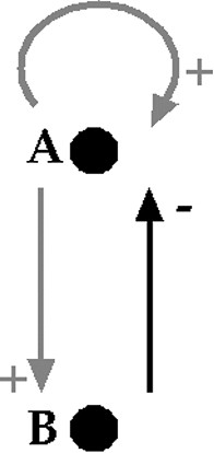
Regulon scheme. Grey arrows are activatory (+) whereas the black one is inhibitory (–). A activates the formation of B and its own formation (self-catalysis), whereas B inhibits the formation of A.

The regulon can have two stable steady states (due to the presence of the positive loop for the multi-attractority and of the negative one for the stability [31,32]). One can note that a Liénard system is a regulon, where A (resp., B) is represented by the variable y (resp., x), if $g, f > 0$ and $- g^{'} + {yf}^{'} < 0$ .

3.4 Examples in cardiac and respiratory coupled systems

To represent the vegetative control system of the cardiac and respiratory functions, let us consider two regulon-type coupled oscillators in interaction [33,34]. Indeed, to simplify, we consider I, a set of inspiratory neurons (a centre firing synchronously with the phrenic nerve) having an self-activatory loop and interacting with E, a set of expiratory neurons (a centre firing during the phrenic silence); E is activated by I (via the pleural stretch receptors) and E inhibits I (through intra-bulbar connections) (Fig. 6).

Fig. 6
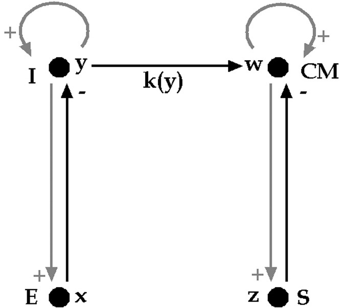
Coupling between the respiratory oscillator (left) and the cardiac oscillator (right).

We neglect in this simplified description other classical groups of neurons corresponding to the Richter classification. Taking them into account leads to a system of higher dimension having the same qualitative dynamical properties, in particular, the entrainment ability [20]. In the same way, by neglecting the peripheral Aschow–Tawara node, we consider the cardiac control system as being made up of two groups of excitable cells, one located in the bulb, composed of neurons and called the cardio-modulator centre CM, and the other located in the heart septum, called the sinusal node S (Fig. 6).

The van der Pol system representing the rhythmic respiratory activity is $d x / d t = y$ , $d y / d t = - x + ε y (1 - x^{2})$ , where ε represents the anharmonic parameter. This oscillator has a free run (proper period) τ equal (near the bifurcation of the van der Pol limit cycle obtained for $ε = 0$ ) to the ratio $τ = 2 π / I$ , where $I = \sqrt{1 - ε^{2} / 4}$ is the imaginary part of the eigenvalues of the Jacobian matrix J of the van der Pol system:

J = [\begin{matrix} 0 & 1 \\ - 1 - 2 ε xy & ε (1 - x^{2}) \end{matrix}]

taken at the stationary point

(x = 0, y = 0)

The van der Pol system representing the rhythmic cardiac activity is $d z / d t = w$ , $d w / d t = - z + η (1 - z^{2}) w + k (y) y$ , where η is the anharmonic parameter and $k (y)$ is the coupling intensity between I and CM. The entrained period of the cardiac oscillator is approximately equal (if η is small) to:

T = 2 π / \sqrt{1 - {(η (1 - (k {(y) y)}^{2}))}^{2} / 4}

Values of ε and η are fixed by the proper periods of the respiratory (4 s) and cardiac (1 s) oscillators. $k (y)$ is obtained by measuring the instantaneous cardiac period T (inter-beats duration) and calculating the slope of the regression line between T and the inspiratory activity $y^{2}$ (y representing the local inspiratory time counted from the beginning of an inspiration, when the cardiac beat of period T is occurring). This slope is approximated by $- π (η k {(y))}^{2} / 2$ , if η and $k (y)$ are small, and is estimated by the correlation coefficient ϱ between T and $y^{2}$ [33,34] multiplied by the ratio between the standard deviations of T and $y^{2}$ . The integrity of the coupling between the two Liénard systems [35] allows the bulbar vegetative control system to adapt to the effort: first, the breathing is entrained by a muscular activity and, secondarily, it entrains the heart. Such a capacity of adaptation disappears in degenerative diseases, like Parkinson or diabetes. Watching a parameter like ϱ is then interesting in elderly people surveillance and at-home watching systems will conversely permit the emergence of a new knowledge about the vegetative regulation and the improvement of at-home rehabilitation systems. More generally, the study of series of coupled oscillators is necessary to explain synchronization, desynchronization, and entrainment phenomena [26]. According to the previous example, we can establish the series of oscillators $i = 1, \dots, N$ :

d x_{i} / d t = y_{i}, d y_{i} / d t = - g (x_{i}) + g (x_{i - 1}) + y_{i} f (x_{i})

The continuous limit in i leads to the partial differential equation (PDE):

\partial^{2} x / \partial t^{2} = f (x) \partial x / \partial t - g^{'} (x) \partial x / \partial s

This new class of PDE is an extension of Burger's equation (by exchanging the role of s and t [36]) and has to be studied in future articles (existence and unicity of solutions, travelling waves, conservative properties...).

4 A toy-model based on microtubules kinetics

Microtubules are major elements of the cell cytoskeleton made of tubular shaped supra-molecular assemblies of a protein, tubulin, of about 20-nm diameter and several micrometres long. Tubulin self-assembles in vitro at 35 °C in presence of a nucleotide, guanosine triphosphate (GTP), giving rise to microtubules. When the reaction begins, microtubules assemble quickly. After a few minutes of reaction, the medium runs low in reactants (tubulin-GTP) and the microtubules become instable. They then start to disassemble. The tubulin-GDP (inactive) liberated by depolymerising microtubules is regenerated into active tubulin-GTP. Progressively, the level of assembly stabilizes and the reaction maintains this level as long as reactants are present. The magnitudes of assembly and disassembly are controlled by the rates of reaction. Kinetics of assembly and disassembly can be described at the ends of individual microtubules by a set of non-linear equations [28]. Realistic global kinetics of microtubule solutions are obtained from populations of reacting individual microtubules. In [28], the assembly was limited by the amount of free tubulin-GTP. The disassembly was linked to the stability of the extremity due to a protecting cap, all at once a particular structural conformation of the protofilaments and a small amount of tubulin-GTP assembled, but not yet hydrolysed.

In the following model, we show that one can express some parts of simplified but realistic kinetics in the form of a Liénard system. Let us assume that x is the length (assembled tubulin concentration) of an individual microtubule, y the concentration of free active tubulin-GTP complexes and z that of the free inactive tubulin-GDP complexes, and that only one of the microtubules extremities is reacting. We also assume that disassembly is at constant rate, the resulting assembly being only regulated by the non-linear assembly kinetics. We obtain the following simplified model:

d x / d t = v_{g} f (y) - k_{s} x

d y / d t = k_{reg} z - v_{g} f (y), d z / d t = k_{s} x - k_{reg} z

where

k_{reg}

is the regeneration rate of tubulin-GDP into tubulin-GTP,

k_{s}

is the constant rate of disassembly of microtubules into tubulin-GDP,

v_{g}

is the maximum reaction rate of microtubule assembly from free tubulin-GTP. The function

f (y)

is a non-linear function that regulates the microtubule assembly; when the amount of free tubulin-GTP is equal to zero,

f (y) = 0

and when it is up to a certain value λ, the function becomes close to 1. The rate of transition between maximum assembly and no assembly is controlled by the non-linearity exponent n. In [28],

f (y)

was a Hill function

f (y) = y^{n} / (λ^{n} + y^{n})

. Such a function can be well fitted by a polynomial function:

f_{p} (y) = 1 - (k_{1} {(1 - ry)}^{m_{1}} - k_{2} {(1 - ry)}^{m_{2}})

, where parameters are chosen to fit well the Hill function. The following parameters were used to simulate the kinetics of the reactive end of the microtubule:

k_{reg} = 0.2 s^{−1}

k_{s} = 0.5 s^{−1}

v_{g} = 20 μm {min}^{−1}

, and the parameters of

f_{p}

were chosen to fit a Hill function with

λ = 2 mg {ml}^{−1}

and

n = 2

. With this set of parameters, which have a pertinent biological signification [28], the simplified model gives a realistic behaviour for one microtubule in an initial environment composed of a limited amount of free tubulin-GTP and tubulin-GDP (Fig. 7).

Fig. 7
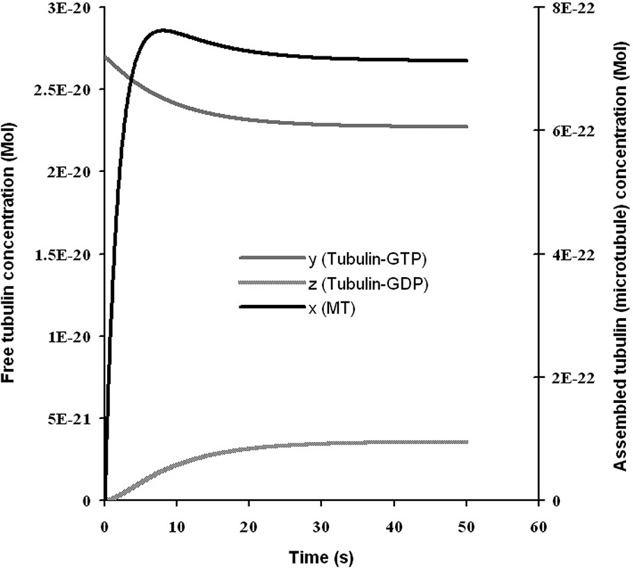
Microtubule kinetics. The three curves are the concentration levels during time of microtubules, tubulin-GTP, tubulin-GDP. Microtubules assemble from tubulin-GTP rapidly. Then, the concentration of tubulin-GTP runs lower and microtubules become unstable and start to disassemble, producing a certain amount of tubulin-GDP, which is rapidly regenerated into tubulin-GTP. With this model, a realistic behaviour of microtubules kinetics is obtained, with a chemical instability after the first phase of rapid assembly, as observed in in vitro experiments.

From this model, we extract three Liénard systems from different reactive conditions :

– when the concentration level of tubulin-GDP is stable ( $d z / d t = 0$ ) (i.e. in biological terms, when the reaction has reached a chemical stationary state or when it is beginning, as to say when no tubulin-GDP has been produced yet), we have:
$d x / d t = v_{g} f_{p} (y) - k_{s} x, d y / d t = k_{s} x - v_{g} f_{p} (y)$
If $w = k_{s} x - v_{g} f_{p} (y)$ , we have:
$d y / d t = w, d w / d t = - w (k_{s} + v_{g} \partial f_{p} (y) / \partial y)$
– when the concentration level of tubulin-GTP is stable ( $d y / d t = 0$ , i.e. at the stationary state of the reaction or in the case of a diluted solution of microtubules without any tubulin regeneration; in this case, the microtubules disassemble and no tubulin-GTP is consumed or produced), we have:
$d x / d t = k_{reg} z - k_{s} x, d z / d t = k_{s} x - k_{reg} z$
If $w = k_{s} x - k_{reg} z$ , we have:
$d z / d t = w, d w / d t = - w (k_{s} + k_{reg})$
– when the concentration level of microtubules is stable ( $d x / d t = 0$ ) (i.e. at the stationary state of the reaction), we have:
$d y / d t = k_{reg} z - v_{g} f_{p} (y) d z / d t = v_{g} f_{p} (y) - k_{reg} z$
If $w = k_{reg} z - v_{g} f_{p} (y)$ , we have:
$d y / d t = w, d w / d t = - w (k_{reg} + v_{g} \partial f_{p} (y) / \partial y)$

Note that, in all cases, the function g is equal to 0 and, in the second case ( $d y / d t = 0$ ), f is constant. All the systems above are susceptible to be decomposed into a potential and a Hamiltonian part. Each of these Liénard systems does not represent the entire microtubule kinetics, but only some parts of the partial reaction kinetics. The potential and Hamiltonian contributions give a better understanding about the manner and the priority by which the reactions run. Indeed, microtubule solutions show very different behaviours, from temporal oscillations to very stable kinetics [37–40]. The potential part of the PH-decomposition of these microtubule Liénard systems gives information on the rate at which the system reaches its stationary state after a perturbation or at the beginning of the reaction. The Hamiltonian part gives information on the parameters driving the system close to its oscillatory behaviour.

5 Extension to metabolic systems

In genetic or metabolic regulatory systems, we can sometimes extract a potential and a Hamiltonian part [1,41]. If we suppose that enzyme kinetics are of Michaelian or allosteric type, a polynomial $P (x_{i})$ exists of order n (called ‘cooperativity’), where $x_{i}$ is the concentration of the substrate catalysed by the ith enzyme of the metabolic system, then the degradation rate of $x_{i}$ is given – if no other metabolite contributes to its catabolism – by $(- \partial \log P (x_{i}) / \partial \log x_{i}) / n$ . In general, the corresponding differential system has a principal potential part (the system tends to become a gradient system when $‖ x_{i} ‖$ tends to infinity [41]), in particular, because of the saturation of terms like $(\partial \log P (x_{i}) / \partial \log x_{i}) / n$ . Then we can prove easily by denoting $y_{i} = \log x_{i}$ (the de Donder chemical affinity [42,43]) that if there are two enzymes in the metabolic system with the same cooperativity n and if the substrate x enters with a constant flux σ, we have:

d y_{1} / d t = \exp (- y_{1}) (σ n - \partial \log P_{1} / \partial y_{1}) / n

d y_{2} / d t = \exp (- y_{2}) (\partial \log P_{1} / \partial y_{1} - \partial \log P_{2} / \partial y_{2}) / n

This system is PH-decomposable into two analytic parts in the neighbourhood of a fixed point or of a just bifurcating limit cycle for which

\exp (- y_{i})

's can be considered as constant, with the potential

P = (\log P_{1} + \log P_{2}) / n

and the Hamiltonian

H = σ y_{2} - \log P_{1} / n

An advantage of this decomposition is the parting of the set of parameters into three distinct families: amplitude-controlling parameters (appearing in P only, like $P_{2}$ parameters), period-controlling parameters (appearing in H only, like σ, which is also involved in the values of the stationary states) and mixed parameters (appearing both in P and H, like $P_{1}$ parameters). Although the PH-decomposition is not unique, this parting of the parameters can be crucial to understand the origin and the control of the cell signalling or tissue morphogenesis.

An example of such an interpretation of the parameters can be given by the high part of the glycolysis centered on the phospho-fructo-kinase (PFK) reaction, which transforms the fructose-6-phosphate (F6P) and the adenosine-tri-phosphate (ATP) into fructose-1,6-di-phosphate (F1,6DP) and adenosine-di-phosphate (ADP) [47]. Let us denote by x (resp. y) the F6P (resp. ADP) concentrations, then because the PFK is an enzyme having an allosteric kinetics (which can be highly non-linear with several plateau features [48]), the equations of the system can be summarized in 2D as [49,50]:

d x / d t = α - F (x, y), d y / d t = ρ (F (x, y) - ν y)

where

F (x, y) = x [{(1 + x)}^{n - 1} {(1 + d y)}^{n} + L_{0} c {(1 + c x)}^{n - 1}] / [{(1 + x)}^{n} {(1 + d y)}^{n} + L_{0} {(1 + c x)}^{n}]

and where the parameters are defined as follows:

α < 1

is the F6P flow coming from the hexokinase reaction (considered as constant), n is the number of PFK regulatory or catalytic subunits (supposed to be the same),

d < 1

is the affinity of ADP (activator) for the regulatory sites of the active PFK,

L_{0}

is the equilibrium constant between active and inactive PFK,

c < 1

is the affinity of the F6P for the catalytic sites of the inactive PFK, and ρ is a time-normalization constant.

Consider now the new variable $X = \sqrt{x}$ , then we have: $d X / d t = (d x / d t) / 2 X$ and, if y remains sufficiently large, we have:

d X / d t \approx - \partial P / \partial X + \partial H / \partial y

d y / d t \approx - \partial P / \partial y - \partial H / \partial X

where

P (X, y) = - (α \log X) / 2 + ρ ν y^{2} / 2 + (\log [{(1 + X^{2})}^{n} {(1 + d y)}^{n} + L_{0} {(1 + c X^{2})}^{n}]) / 4 n

and

H (X, y) = - ρ (\log [{(1 + X^{2})}^{n} {(1 + d y)}^{n} + L_{0} {(1 + c X^{2})}^{n}]) / 4 n

The system presents a limit cycle (cf. Fig. 8), which bifurcates from the unstable stationary state ( $x_{s s} = F {(., y_{s s})}^{−1} (α)$ , $y_{s s} = α / ν$ ) for the condition [41]:

{(\partial F (x_{s s}, y_{s s}) / \partial x - ν)}^{2} + {(\partial F (x_{s s}, y_{s s}) / \partial y)}^{2} - 2 ν \partial F (x_{s s}, y_{s s}) / \partial y - 2 \partial F (x_{s s}, y_{s s}) / \partial x . \partial F (x_{s s}, y_{s s}) / \partial y < 0

where (after [48])

\partial F (x_{s s}, y_{s s}) / \partial x = (\partial D / \partial x (D - x \partial D / \partial x) + x D \partial^{2} D / \partial x^{2}) / n D^{2}

with

D = {(1 + x)}^{n} {(1 + d y)}^{n} + L_{0} {(1 + c x)}^{n}

\partial D / \partial x = n [{(1 + x)}^{n - 1} {(1 + d y)}^{n} + L_{0} c {(1 + c x)}^{n - 1}]

\partial^{2} D / \partial x^{2} = n (n - 1) [{(1 + x)}^{n - 2} {(1 + d y)}^{n} + L_{0} c^{2} {(1 + c x)}^{n - 2}]

and

\partial F (x_{s s}, y_{s s}) / \partial y = n d {(1 + d y)}^{n - 1} L_{0} x {(1 + c x)}^{n - 1} {(1 + x)}^{n - 1} (1 - c) / D^{2}

which holds when

ν = \partial F (x_{s s}, y_{s s}) / \partial x

and when y remains sufficiently large. Then the parameters α and ν are controlling the amplitude of the ADP signal, ρ is controlling the frequency of the ADP signal, whereas n, c and d are mixed.

Fig. 8
Limit-cycle that represents the high part of the glycolysis driven by the phospho-fructo-kinase, as described before. The parameters used for the limit cycle simulation are equal to: $L_{0} = 3 \times 10^{3}$ , n=3, c=0.02, d=1, ν=0.01, logρ=3, and logα=−1. Period=7.096.

6 Conclusion

In a first note [1], we developed a new method for algebraically approximating limit cycles of classical dynamical systems like n-switches, Lotka–Volterra and Liénard systems, allowing one to separate the flow into two parts, a dissipative one, called potential (or gradient), and a conservative one, called Hamiltonian, whose parameters have different roles, with more amplitude modulating in the dissipative part and more frequency modulating in the conservative one. The specific power of each parameter will be evaluated in the future from generalization of the control strengths, currently available only in case of stationary states or of relaxation oscillations [44–46]. It will allow a practical use of the present approach in all biological applications described in this paper and in others of the same type in narrow fields (population dynamics, genetic control, immunologic response...).

Acknowledgements

We are very indebted to A. Winfree (deceased in November 2002) for having introduced the notion of isochron and for having given one of the first convincing examples of application of dynamical systems theory in biology, and to J.-P. Françoise for stimulating discussions and helpful suggestions.

Bibliographie

[1] J. Demongeot, N. Glade, L. Forest, Liénard systems and potential-Hamiltonian decomposition – I. Methodology, II. Algorithm and III. Applications, C. R. Acad. Sci. Paris, Ser. I, in press

[2] O. Cinquin; J. Demongeot High-dimensional switches and the modeling of cellular differentiation, J. Theor. Biol., Volume 233 (2005), pp. 391-411

[3] U. Kling; G. Székely Simulation of the rhythmic nervous activities, Kybernetik, Volume 3 (1968), pp. 89-103

[4] A. Turing The mathematical basis of morphogenesis, Phil. Trans. R. Soc. Lond. B, Volume 237 (1952), pp. 37-47

[5] A.N. Kolmogorov; I. Petrowski; N. Piskounov Étude de l'équation de la diffusion avec croissance de la quantité de matière et son application à un problème biologique, Mosc. Univ. Bull. Math., Volume 1 (1937), pp. 1-25

[6] J. Demongeot; R. Thomas; M. Thellier A mathematical model for storage and recall functions in plants, C. R. Acad. Sci. Paris, Ser. III, Volume 323 (2000), pp. 93-97

[7] M. Thellier; J. Demongeot; J. Guespin; C. Ripoll; V. Norris; R. Thomas A logical (discrete) formulation model for the storage and recall of environmental signals in plants, Plant Biol., Volume 10 (2004), pp. 1055-1075

[8] J. Demongeot; M. Thellier; R. Thomas Storage and recall of environmental signals in a plant: modelling by use of a differential (continuous) formulation, C. R. Biologies, Volume 329 (2006), pp. 971-978

[9] A. Jolliot; A. Prochiantz Transduction peptides: from technology to physiology, Nat. Cell Biol., Volume 6 (2004), pp. 189-196

[10] L. Forest; J. San Martin; F. Padilla; F. Chassat; F. Giroud; J. Demongeot Cellular modelling of secondary radial growth in conifer trees: application to Pinus radiata, Acta Biotheor., Volume 52 (2004), pp. 415-438

[11] A.I. Khibnik; B. Krauskopf; C. Rousseau Global study of a family of cubic Liénard equations, Nonlinearity, Volume 11 (1998), pp. 1505-1519

[12] N.G. Lloyd Liénard systems with several limit cycles, Math. Proc. Cambridge Philos. Soc., Volume 102 (1987), pp. 565-572

[13] N.G. Lloyd; S. Lynch Small-amplitude limit cycles of certain Liénard systems, Proc. R. Soc. Lond. A, Volume 418 (1988), pp. 199-208

[14] S. Lynch Small-amplitude limit cycles of Liénard systems, Calcolo, Volume 27 (1990), pp. 1-32

[15] S. Lynch Liénard systems and the second part of Hilbert's 16th problem, Non-Linear Anal., Volume 30 (1997), pp. 1395-1403

[16] T.R. Blows; N.G. Lloyd The number of small-amplitude limit cycles of Liénard equations, Math. Proc. Cambridge Philos. Soc., Volume 95 (1984), pp. 359-366

[17] J. Aracena; J. Demongeot; E. Goles Fixed points and maximal independent sets on AND–OR networks, Discr. Appl. Math., Volume 138 (2004), pp. 277-288

[18] J. Aracena; J. Demongeot; E. Goles On limit cycles of monotone functions with symmetric connection graphs, Theoret. Comput. Sci., Volume 322 (2004), pp. 237-244

[19] B. van der Pol; J. van der Mark The heartbeat considered as a relaxation oscillation and an electrical model of the heart, Philos. Mag., Volume 6 (1928), pp. 763-775

[20] T. Pham Dinh; J. Demongeot; P. Baconnier; G. Benchetrit Simulation of a biological oscillator: the respiratory rhythm, J. Theor. Biol., Volume 103 (1983), pp. 113-132

[21] J. Nagumo, S. Arimoto, S. Yoshizawa, An active pulse transmission line simulating nerve axons, in: Proc. IRL 50, 1960, pp. 2061–2070

[22] R. FitzHugh Impulses and physiological states in theoretical models of nerve membranes, Biophys. J., Volume 1 (1961), pp. 445-466

[23] A.L. Hodgkin; A.F. Huxley A quantitative description of membrane current and its application to conduction and excitation in nerve, J. Physiol., Volume 117 (1952), pp. 500-544

[24] R. Thom Topological models in biology, Topology, Volume 8 (1969), pp. 313-335

[25] C. Zeeman Differential equations for the heartbeat and nerve impulse, Dynamical Systems Symposium Univ. Bahia, Academic Press, New York, 1973, pp. 683-741

[26] A. Tonnelier; S. Meignen; H. Bosch; J. Demongeot Synchronization and desynchronization of neural oscillators: comparison of two models, Neural Networks, Volume 12 (1999), pp. 1213-1228

[27] J. Demongeot; M. Kaufmann; R. Thomas Positive feedback circuits and memory, C. R. Acad. Sci. Paris, Ser. III, Volume 323 (2000), pp. 69-79

[28] N. Glade; J. Demongeot; J. Tabony Numerical simulations of self-organisation in microtubule solutions by reaction–diffusion processes, Acta Biotheor., Volume 50 (2002), pp. 239-268

[29] P. Glansdorff; I. Prigogine Thermodynamic Theory of Structure, Stability and Fluctuations, Wiley, New York, 1971

[30] J.J. Tyson The Belousov–Zhabotinskii reaction, Lect. Notes Biomaths, Volume 10 (1976)

[31] O. Cinquin; J. Demongeot Positive and negative feedback: striking a balance between necessary antagonists, J. Theor. Biol., Volume 216 (2002), pp. 229-241

[32] O. Cinquin; J. Demongeot Positive and negative feedback: mending the ways of sloppy systems, C. R. Biologies, Volume 325 (2002), pp. 1085-1095

[33] J. Demongeot; G. Virone; F. Duchêne; G. Benchetrit; T. Hervé; N. Noury; V. Rialle Multi-sensors acquisition, data fusion, knowledge mining and alarm triggering in health smart homes for elderly people, C. R. Biologies, Volume 325 (2002), pp. 673-682

[34] S. Ben Lamine; P. Calabrese; H. Perrault; T.P. Dinh; A. Eberhard; G. Benchetrit Individual differences in respiratory sinus arrhythmia, Am. J. Physiol. Heart Circ. Physiol., Volume 286 (2004), pp. 2305-2312

[35] J.D. Murray Mathematical Biology, Springer, Berlin, 1989

[36] S. Thibault; L. Heyer; G. Benchetrit; P. Baconnier Ventilatory support: a dynamical systems approach, Acta Biotheor., Volume 50 (2002), pp. 269-279

[37] F. Pirollet; D. Job; R.L. Margolis; J.R. Garel An oscillatory mode for microtubule assembly, EMBO J., Volume 6 (1987), pp. 3247-3252

[38] M.-F. Carlier; R. Melki; D. Pantaloni; T.L. Hill; Y. Chen Synchronous oscillations in microtubule polymerisation, Proc. Natl Acad. Sci. USA, Volume 84 (1987), pp. 5257-5261

[39] E. Mandelkow; E.M. Mandelkow; H. Hotani; B. Hess; S.C. Muller Spatial patterns from oscillating microtubules, Science, Volume 246 (1989), pp. 1291-1293

[40] B. Houchmandzadeh; M. Vallade Collective oscillations in microtubule growth, Phys. Rev. E, Volume 53 (1996), pp. 6320-6324

[41] J. Demongeot Existence de solutions périodiques pour une classe de systèmes différentiels gouvernant la cinétique de chaînes enzymatiques oscillantes, Lect. Notes Biomaths, Volume 41 (1981), pp. 40-62

[42] T. de Donder Thermodynamic Theory of Affinity: A Book of Principles, Oxford University Press, Oxford, UK, 1936

[43] T. de Donder, Sur la théorie des invariants intégraux, Ph.D. thesis, ULB, Brussels, 1899

[44] P. Baconnier; P. Pachot; J. Demongeot An attempt to generalize the control coefficient concept, J. Biol. Syst., Volume 1 (1993), pp. 335-347

[45] J. Demongeot; F. Esteve; P. Pachot Comportement asymptotique des systèmes : applications en biologie, Rev. Int. Syst., Volume 2 (1988), pp. 417-442

[46] P. Ruoff; M.K. Christensen; J. Wolf; R. Heinrich Temperature dependency and temperature compensation in a model of yeast glycolytic oscillations, Biophys. Chem., Volume 106 (2003), pp. 179-192

[47] J. Demongeot; N. Kellershohn Glycolytic oscillations: an attempt to an ‘in vitro’ reconstitution of the higher part of glycolysis, Lect. Notes Biomaths, Volume 49 (1983), pp. 17-31

[48] J. Demongeot; M. Laurent Sigmoidicity in allosteric models, Math. Biosci., Volume 67 (1983), pp. 1-17

[49] E.E. Sel'kov Self-oscillations in glycolysis. 1. A simple kinetic model, Eur. J. Biochem., Volume 4 (1968), pp. 79-86

[50] A. Goldbeter; R. Lefever Dissipative structures for an allosteric model. Application to glycolytic oscillations, Biophys. J., Volume 12 (1973), pp. 1302-1315

Commentaires - Politique

Ces articles pourraient vous intéresser

Liénard systems and potential-Hamiltonian decomposition III – applications

Nicolas Glade; Loic Forest; Jacques Demongeot

C. R. Math (2007)

Liénard systems and potential-Hamiltonian decomposition II – algorithm

Jacques Demongeot; Nicolas Glade; Loic Forest

C. R. Math (2007)

Liénard systems and potential-Hamiltonian decomposition I – methodology

Jacques Demongeot; Nicolas Glade; Loic Forest

C. R. Math (2007)