

1 Introduction
Monogonont rotifera are small invertebrate animals that inhabit aquatic media. These species of rotifera have males and females and their reproduction cycle, named Cyclic Parthenogenesis, which is a combination of sexual and asexual reproduction (two phases), has a considerable interest and provides a valuable model for the study of sex allocation [2].
The first phase is asexual with no male presence. It begins after the hatching of resting eggs that become amictic females. Then, there are only amictic females producing diploid eggs that hatch right away to become new amictic females.
The second phase begins induced by environmental factors, there is sexual reproduction and it takes place simultaneously with the other phase. The amictic females begin to produce amictic daughters and mictic (sexual) ones. The virgin mictic daughters produce haploid eggs when they reach maturity, these eggs become haploid males after hatching. The males can fertilize the virgin mictic females in the few hours of life of these ones. And, the mated mictic females (the mictic females fertilized) produce resting eggs and the reproductive cycle begins again. More information about this reproduction cycle can be found in [3,4].
The model for the sexual phase of monogonont rotifera, presented in [5], involves three subclasses in the population: virgin mictic females (male-producing), mated mictic females (resting eggs producing) and haploid males.
This problem has been modelled by means of a non-linear age-structured population model. In the following, we try to explain the reasons that led the modellers to make this choice. The structured population modelling combines the knowledge about the individual, its basic unit, and the study of the higher organizational level: the population. In other words, its aim is to know how the individual variability influences the dynamics of the whole population, usually conceived as a frequency distribution of individuals that evolves over time. This variability is introduced into the model ‘structuring’ the population, i.e. classifying the individuals by some (continuous) internal variables as age (also, size, energy reserves or whatever variable(s) that reflects it and has an actual influence in the population dynamics). On the other hand, non-linearities enable us to take into account the influence of the population dynamics in the individuals' life history.
In [1], Calsina et al. made a theoretical study of such a model showing a unique stationary population density that is stable as long as a parameter, related to male–female encounter rate, remains below a critical value. Also, they obtained that the stationary solution becomes unstable and a limit cycle appears, when the parameter increases beyond the critical value. They thought that a study of this unstable equilibrium case from the evolutionary point of view, in order to obtain a better approach to this limit cycle, could be done numerically. The present paper is devoted to carry out such a study.
Models such as those that we are going to introduce often cannot be solved analytically, and require numerical integration to obtain an approximation for the solution.
The numerical integration of age-structured models has been studied in several references during the last two decades. In the following, we make a brief overview of the numerical integration techniques used to solve non-linear models related to the Gurtin–MacCamy one. Kostova [6] used the discretized method of lines in order to apply it to a special case of the Gurtin–MacCamy method. Schemes based on upwind discretization were analysed by López-Marcos [7] and second-order numerical schemes using the box method were considered by Fairweather and López-Marcos [8,9]. However, the most popular technique to integrate numerically such type of problems is the characteristics method: Douglas and Milner [10] (explicit first-order schemes, with linear boundary conditions), Chichia Chiu [11], Kostova [12] (for a model describing interacting population dynamics), Kwon and Cho [13] and Milner and Rabbiolo [14] (explicit two-step methods based on the central difference operator along characteristics with fertility rate independent of the total size of the population). The latter authors also considered their numerical method for the numerical solution of a two-sex model, and analysed for linear models an explicit fourth-order method based on the classical fourth-order Runge–Kutta method. These methods are generalized in Abia and López-Marcos [15] (numerical methods of arbitrary order based on general Runge–Kutta methods are analysed). Integration along characteristics by means of a representation of the theoretical solution was introduced by Abia and López-Marcos [16] where implicit second-order schemes based on Padé rational approximations for the exponential were analysed. The use of two-step methods (such as which was done by Milner and Rabbiolo [14] and Kwon and Cho [13]) joint with open quadrature rules is presented in [17] to obtain explicit numerical second-order methods.
It should be noted that several numerical methods have been successfully applied to real life populations in the past, such as intramolluscan trematode populations [18], the Nicholson's blowflies (L. curpina) and the gray squirrel population (Sciurus carolinensis) [19] (also in demography [14]). Favorable comparisons between the application of such schemes and models to populations indicate that they are valid tools to investigate biological systems. A more detailed revision on the numerical integration of age-structured population models can be founded in [20] and for size-structured models we refer to [21].
In this paper, we present the numerical investigation on the solution of the model that describes the dynamics of the sexual phase of monogonont rotifera. Also, we get numerically a better approach to the limit cycle that the linear approximation obtained in [1]. This is made with different parameter values and distinct initial conditions. We will consider both the stable and the unstable equilibrium cases. In addition, in the unstable equilibrium case, we study the evolution to the (stable) limit cycle. On the other hand, we obtain the density distribution of the population for the stable equilibrium and also for different stages of the limit cycle.
2 Formulation of the model
The population densities satisfy the following system of integro-differential equations that are based on the balance law of the population:
| (1) |
The equation of mated mictic females can be considered separately whenever the other two equations have been solved. Also, as in [1], a rescaling to reduce the number of parameters is introduced:
| (3) |
| (4) |
| (5) |
3 Numerical method
From a numerical point of view, the model (3)–(5) has meaningful difficulties to keep in mind. First, the model consists on a system of partial differential equations; second, the model is a non-linear one; and finally, these non-linearities are caused by non-local terms. So, the design of a numerical method that solves that problem, its computational implementation and the corresponding convergence analysis are not straightforward tasks. Due to the fine behavior of the numerical method studied in [22] for physiologically structured population models, we have made suitable (and significant) changes on it to treat numerically the problem (3)–(5). The scheme designed is implicit and second-order accurate.
The problem is integrated in a fixed time interval [0,Tf] and we also consider a finite maximum age Amax, which is chosen sufficiently large to make a realistic simulation.
The method that we are going to use integrates the model along the characteristic curves. In this case, the solutions of (3) have the following property: for each a0, with 0<a0<Amax, and such that a0+k<Amax, then
| (6) |
| (7) |
Now, we are going to describe the numerical method. Given a positive integer J, we define k=Amax/J (recall that we have considered a maximum age Amax) and we introduce a uniform partition of the interval [0,Amax], aj=jk, 0⩽n⩽J. We define the discrete time levels, tn=nk, 0⩽n⩽N, where N=[Tf/k].
We refer to the grid point aj by a subscript j and to the time level tn by a superscript n. Let Vjn and Hjn be a numerical approximation to v(aj,tn) and h(aj,tn), respectively, 0⩽j⩽J, 0⩽n⩽N; we also denote , , 0⩽n⩽N, and with the composite trapezoidal quadrature rule
Now, we suppose that approximations to the initial conditions given in (5). Then, the general recursion of the method is the following. Suppose that , 0⩽n⩽N−1, are known. Next, we obtain approximations Vn+1j+1 and Hn+1j+1 to v(xj+1,tn+1) and h(xj+1,tn+1) for 0⩽j⩽J−1, 0⩽n⩽N−1, by means of the following discretization of the representation formulae (6), (7):
| (8) |
| (9) |
| (10) |
| (11) |
To solve the non-linear equations (8)–(11), we have used an iterative method. If the numerical solution (V0n,…,VJn), (H0n,…,HJn), n⩾0, is known, we obtain the values (V0n+1,…,VJn+1), (H0n+1,…,HJn+1), by means of the following algorithm:
STEP 1
For each m⩾0,
For each 0⩽j⩽J−1, m⩾0,
For each j, 0⩽j⩽J−1,
If for any j, 1⩽j⩽J,
END
In the above iterative procedure, steps 1 and 2 are made only once at the beginning of the algorithm. This iterative procedure has showed its efficiency in some previous works such as [15,16,22–24].
We do not present the convergence analysis of the method because the tools and the arguments needed are completely similar to those ones used in [16]. The only added difficulty of such analysis may be the complexity of the numerical scheme in terms of the notation of variables we need because we are integrating a system of partial differential equations. However, the analysis of the present model, which is age-structured, does not have the inherent complexity of a size-structured model as that considered in [22]. We refer to [25] in order to take into account the effect of the singularities of the solution on the accuracy of the numerical method.
4 Numerical experimentation
We have carried out an extensive numerical experimentation with the scheme introduced in the previous section. We have used different initial conditions and distinct parameter values in the numerical integration of the problem, although in this paper we present the most significant results.
The integration has been made for the value Tf=50 and the maximum age Amax=37. In all cases we are going to present, we have used the next parameter values μ=0.9355, δ=1.4463 and T=0.4274. For this choice, the equilibrium becomes unstable for values of E, the male–female encounter rate, greater than the critical value Eun=501.832 (see [1], for more details). We report the results obtained with the step size k=0.0074 and we present them by means of several figures.
We have chosen a first set of initial conditions that are really far from the equilibrium and from the limit cycle, for the two possible situations: stable or unstable equilibrium, respectively. With these numerical experiments, we show the robustness of our numerical method, because it always reaches the target (equilibrium or limit cycle). Next, we have taken two set of initial conditions that are closer to the equilibrium (and, also, the limit cycle). The first one is located outside the limit cycle and the other one inside it, whenever the male–female encounter rate E satisfies E>Eun. In all cases, we show that the solution of the numerical method reaches the desired aims. In addition, the limit cycle (E>Eun) appears to have, at least numerically, a stable behaviour.
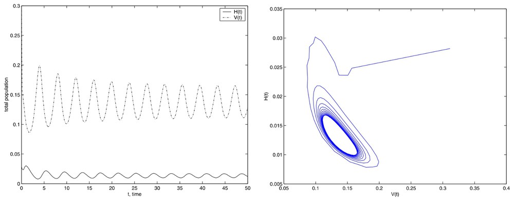
For each initial condition set, we show the results with two values of E, one of them belonging to a stable equilibrium case and the other to an unstable one. The simulations for each case are presented using a couple of figures. The left-hand figure shows the evolution of the two populations, H(t) and V(t), along time. In this graph, we show the time in the x-axis and the total quantity of both population (H(t) and V(t)) in the y-axis. We use a solid line (−) to draw H(t) and a hyphen-dotted line (−.) to draw V(t). In the right-hand figure, we present the evolution of (H(t),V(t)), for t∈[0,Tf].
To begin with, we present the numerical results obtained for the remote initial conditions set: (12)
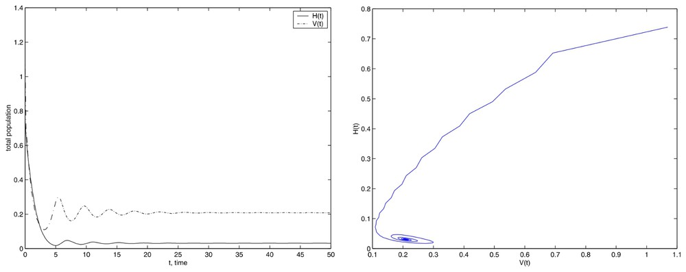
Simulations with the initial conditions set (12) and E=200.
The attractive character of the equilibrium is apparent. We have obtained the same behavior in experiments carried out with other different values of E, E<Eun.
For the other case, we have used E=675.84, the simulation is shown in Fig. 2. We see the limit cycle, that appears to be stable. We have to note that, in the second graph, we have plotted the values corresponding to t∈[3.7,50], in other case we cannot appreciate the limit cycle (recall that the initial conditions are far from the limit cycle and for this situation, the dimensions of the figure are small). Again, we have tried with different values of E, E>Eun and we have obtained the same results. With this two first examples, we show the robustness of the numerical method because we get both the stable equilibrium and the stable limit cycle beginning from remote initial conditions.
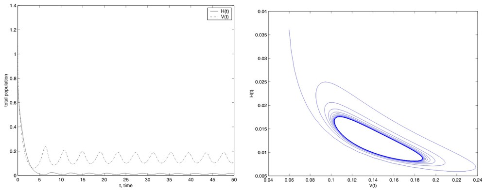
Simulations with the initial conditions set (12) and E=675.84.
Next, we are going to use nearer initial conditions to the aims. The first one is located outer the limit cycle, when it exists. We put
| (13) |
For the stable equilibrium case, we have used the value E=500 a nearby Eun value. The numerical results with Tf=50, showed in Fig. 3, could lead us to think that numerically the equilibrium could be unstable due to the possible appearance of the limit cycle.
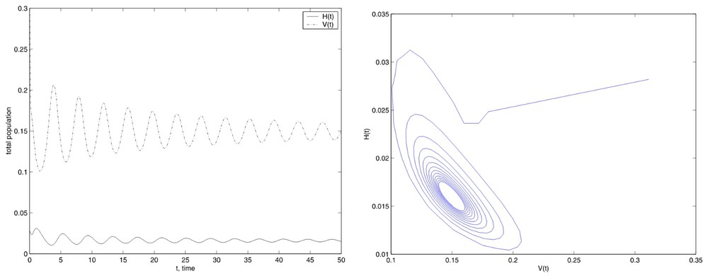
Simulations with the initial conditions set (13), Tf=50 and E=500.
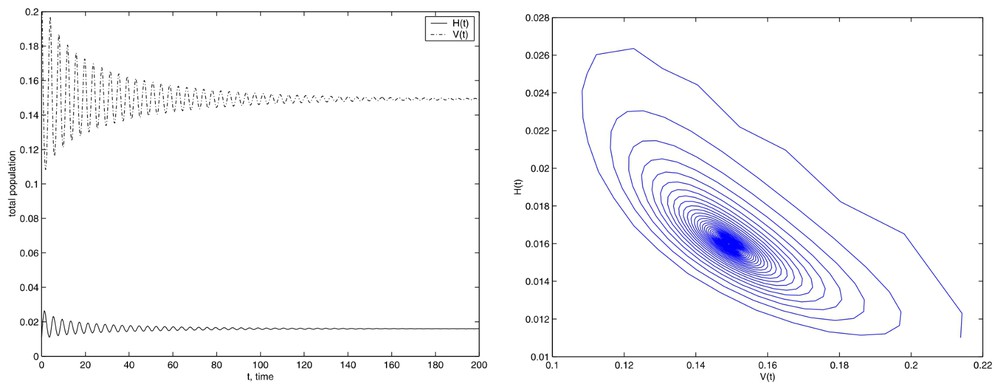
However, Fig. 4, in which graphs we have used the same E value and a larger Tf value, Tf=200, shows the stability of such equilibrium.
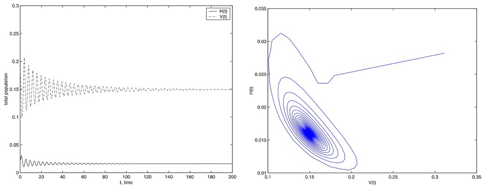
Simulations with the initial conditions set (13), Tf=200 and E=500.
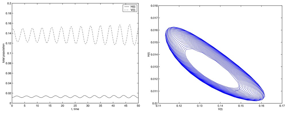
Then we have to take care about the numerical integration, because it could lead to wrong conclusions if the integration parameters, such as the final time of computation, are not suitable for the dynamical properties of the problem. Again, the numerical method shows its nice properties because the integration for a long time is carried out successfully. On the other hand, if we use E=675.84, we get the limit cycle that appears to be stable, as shown in Fig. 5. We have also employed with different values of E, greater or less than Eun with the same results.
Simulations with the initial conditions set (13) and E=675.84.
Finally, we present the numerical simulations where we have used initial conditions located inside the limit cycle, whenever it exists. We take:
| (14) |
Simulations with the initial conditions set (14) and E=675.84.
Although, when we use a value lower than the critical value the stable equilibrium appears. In this case, we present in Fig. 7 the results obtained with E=500.
Simulations with the initial conditions set (14), Tf=200 and E=500.
The numerical simulations not only show the dynamics of the problem but also get the age structure of the population density of virgin mictic females (v(a,t)) and haploid males (h(a,t)). This fact enables us to know the age structure of the stable equilibrium and that of the limit cycle. In Figs. 8 and 9, we show the age in the x-axis and the population density in the y-axis. The range of the age variable used in the figures is [0,4] instead of [0,37], because the population density is not significant for greater values of such variable. We draw v(a,Tf) by means a solid line (−) and h(a,Tf) by means an hyphen-dotted line (−.).
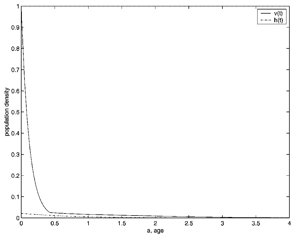
Age structure of the population densities in the equilibrium state.
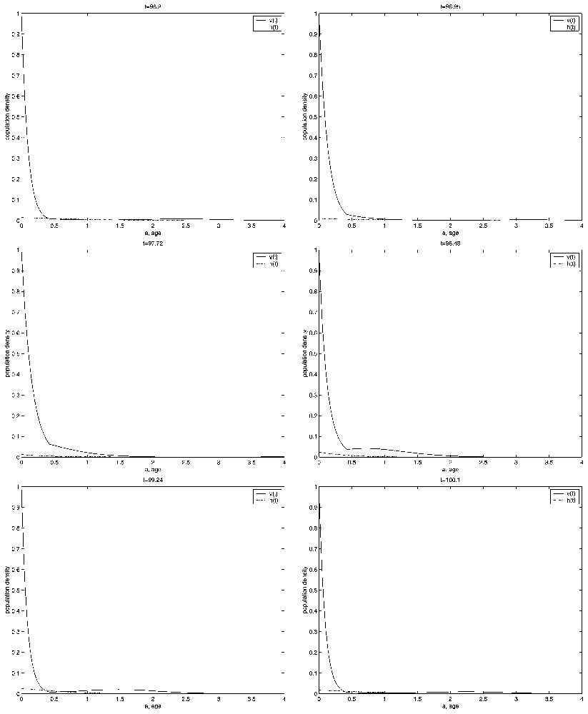
Age structure of the population densities for different values of a period of the limit cycle.
First, in Fig. 8, we show the population age structure when the equilibrium is reached. We have taken E=500. And, finally, we present in Fig. 9 the evolution in time of the distribution density of both populations in one period of the limit cycle. Taking E=675.84, we show the age structure of both populations at time values t=96.2, t=96.95, t=97.72, t=98.48, t=99.24, and t=100.1 (note that in this case the period is near to 3.91).
Another matter that we have to take into account is that the graphs in Figs. 8 and 9 show a discontinuity in the first derivative of the v(t) age-structured population at the threshold fertilization age T, which our numerical method is able to obtain. This discontinuity is theoretically shown for the equilibrium state in [1], but we show that it also appears in the case of the stable limit cycle, which is in agreement with the first equation of (3), because its right-hand side involves the characteristic function of the interval [0,T].
5 Discussion
We have studied the numerical integration of a model that describes the sexual phase of monogonont rotifera reproduction proposed in [1].
We have shown the robustness and the reliability of our numerical method by means of numerical experiments that cover different situations. The scheme is so robust that it is able to get the solutions for longer time intervals and also it can obtain discontinuities of the first derivative of the distribution of virgin mictic females. We have also shown that the method can be used to analyse the dynamics of the populations when the values of the encounter male–female rate E is close to its critical value Eun.
The results of our numerical study are in agreement with the theoretical results derived in [1], and obtain the age structure of the populations for the stable limit cycle [20,21,25].
Acknowledgements
The authors are supported in part by project DGESIC-JGES BFM2002-01250 and projects VA002/01 and VA063/04 (Cousefería de Educación y Cultura de la Junta de Castilla y León).