A hierarchical matrix model to assess the impact of habitat fragmentation on population dynamics: an elasticity analysis

Jean-Baptiste Pichancourt; Françoise Burel; Pierre Auger

doi:10.1016/j.crvi.2005.09.009

Biological modelling / Biomodélisation

A hierarchical matrix model to assess the impact of habitat fragmentation on population dynamics: an elasticity analysis
[Un modèle matriciel hiérarchisé pour estimer l'impact de la fragmentation des habitats sur la dynamique des populations : une analyse d'élasticité]

Présenté par : Michel Thellier

Jean-Baptiste Pichancourt ¹ ; Françoise Burel ¹ ; Pierre Auger ²

¹ UMR ECOBIO CNRS, université Rennes-1, bât. 14b, campus de Beaulieu, 35042 Rennes cedex, France
² Centre IRD Île-de-France, 32, av. Henri-Varagnat, 93143 Bondy cedex, France

Comptes Rendus. Biologies, Volume 329 (2006) no. 1, pp. 31-39.

Résumés

Anglais
Français

To better understand the role of habitat quality and boundaries on population dynamics at the landscape scale, we develop a model combining a spatially implicit approach, a spatial population Leslie-type model and an implicit model of habitat fragmentation. An original approach of elasticity permits to identify which types of element and boundary influence the most population viability according to the wood fragmentation degree. The studied species is a corridor forest insect sensitive to fragmentation (Abax parallelepipedus, Coleoptera, Carabidae). We show that a single large patch of wood is better than several small patches for the population viability.

Pour mieux comprendre le rôle de la qualité des éléments et de leurs lisières sur la dynamique de population à l'échelle du paysage, nous utilisons un modèle combinant un sous-modèle implicite de paysage, un sous-modèle matriciel de Leslie spatialisé, ainsi qu'un sous-modèle implicite de fragmentation du paysage. Nous introduisons une approche originale de l'élasticité pour savoir quel type d'élément et de lisière influence le plus la viabilité de la population en fonction du degré de fragmentation. L'espèce étudiée est un insecte forestier sensible à la fragmentation (Abax parallelepipedus, Coleoptera, Carabidae). Nous montrons qu'un seul grand patch de bois est meilleur que plusieurs petits.

Métadonnées

Reçu le : 2005-09-02
Accepté le : 2005-09-30
Publié le : 2005-12-02

PMID

DOI : 10.1016/j.crvi.2005.09.009

Keywords: Abax parallelepipedus, Wood fragmentation, Spatial Leslie-type model, Time scales, SLOSS, Asymptotic population growth rate, Elasticity analysis
Mot clés : Abax parallelepipedus, Fragmentation de l'habitat, Modèle de Leslie spatialisé, Échelles de temps, SLOSS, Taux d'accroissement asymptotique, Analyse d'élasticité

Affiliations des auteurs :

Jean-Baptiste Pichancourt ¹ ; Françoise Burel ¹ ; Pierre Auger ²

¹ UMR ECOBIO CNRS, université Rennes-1, bât. 14b, campus de Beaulieu, 35042 Rennes cedex, France
² Centre IRD Île-de-France, 32, av. Henri-Varagnat, 93143 Bondy cedex, France

@article{CRBIOL_2006__329_1_31_0,
     author = {Jean-Baptiste Pichancourt and Fran\c{c}oise Burel and Pierre Auger},
     title = {A hierarchical matrix model to assess the impact of habitat fragmentation on population dynamics: an elasticity analysis},
     journal = {Comptes Rendus. Biologies},
     pages = {31--39},
     publisher = {Elsevier},
     volume = {329},
     number = {1},
     year = {2006},
     doi = {10.1016/j.crvi.2005.09.009},
     language = {en},
}

TY  - JOUR
AU  - Jean-Baptiste Pichancourt
AU  - Françoise Burel
AU  - Pierre Auger
TI  - A hierarchical matrix model to assess the impact of habitat fragmentation on population dynamics: an elasticity analysis
JO  - Comptes Rendus. Biologies
PY  - 2006
SP  - 31
EP  - 39
VL  - 329
IS  - 1
PB  - Elsevier
DO  - 10.1016/j.crvi.2005.09.009
LA  - en
ID  - CRBIOL_2006__329_1_31_0
ER  -

%0 Journal Article
%A Jean-Baptiste Pichancourt
%A Françoise Burel
%A Pierre Auger
%T A hierarchical matrix model to assess the impact of habitat fragmentation on population dynamics: an elasticity analysis
%J Comptes Rendus. Biologies
%D 2006
%P 31-39
%V 329
%N 1
%I Elsevier
%R 10.1016/j.crvi.2005.09.009
%G en
%F CRBIOL_2006__329_1_31_0

Jean-Baptiste Pichancourt; Françoise Burel; Pierre Auger. A hierarchical matrix model to assess the impact of habitat fragmentation on population dynamics: an elasticity analysis. Comptes Rendus. Biologies, Volume 329 (2006) no. 1, pp. 31-39. doi : 10.1016/j.crvi.2005.09.009. https://comptes-rendus.academie-sciences.fr/biologies/articles/10.1016/j.crvi.2005.09.009/

Version originale du texte intégral

1 Introduction

Landscapes (‘heterogeneous land area composed of cluster of interacting ecosystems’ [1]) are heterogeneous and dynamic. The way quality and spatial structure of landscapes evolved since 1950s endanger a large number of species under the influence of human activities (by alterations of human land use pattern, industrial activity, and agriculture) or natural disturbances. Habitat fragmentation is one of the major causes of this biodiversity erosion [2–4]. In this context, specialist species, that is, those using only one land cover type, have been abundantly studied because they are sensitive to habitat fragmentation [5]. Metapopulation models are adapted for specialist species and are abundantly used to assess the effect of habitat fragmentation on population dynamics. However, some effects of the spatial landscape structure cannot explicitly be studied via metapopulation models [6]: they do not consider effects of neighbouring elements (e.g., element: distinct ecosystems that make up a landscape) on characteristics and dynamics of a particular patch of ‘suitable element’ (i.e. ‘habitat’), they cannot assess the impact of boundaries on movements of organisms and processes both within and between elements. Finally, they cannot consider the effect of spatial and temporal variation of element quality on population dynamics. SEPMs (Spatial Explicit Population Models: see [7] for definition and applications) permit to better consider spatial heterogeneity in its continuity and its complexity and link landscape structure with population dynamics. They are designed for given landscapes, but results are difficult to transfer to other types of landscapes. On the other hand, some SIPMs (spatially implicit population models) permit to identify general patterns linking population and landscape [8–10] while loosing accuracy on spatial structure. So in order to assess the response of a population according to habitat fragmentation, we develop a generic model that combines an implicit landscape model, a spatial population Leslie-type model and an implicit model of habitat fragmentation. The model of habitat fragmentation is divided in two sub processes: habitat loss and breaking apart of habitat (habitat fragmentation per se) [4]. This distinction allows determining ‘how much habitat is enough?’ [4]. Or for a given proportion of habitat, what kind of spatial management must be maintained: a “single large or several small” (SLOSS) patches of habitat? [11,12]. The goal of this study is also to determine the relative contributions (i.e. elasticity) of the different elements and boundaries (at local scale) to population viability (at the landscape scale), according to habitat fragmentation. We present an application to a corridor forest species sensitive to woody element fragmentation at the landscape scale [13,14] Abax parallelepipedus (Coleoptera: Carabidae). We finally discuss the interest of our modelling approach in comparison with individual-based models (IBMs) and metapopulation models, which consider the landscape.

2 Material and methods

2.1 Biology of A. parallelepipedus

A. parallelepipedus is a common insect (Coleoptera: Carabidae) of the temperate forests in Europe [15] and eastern Canada [16,17]. Adult length ranges from 16 to 22 mm. It lives under bracken [18], in moss, on clusters of dead leaves and stones [19]. A. parallelepipedus belongs to the group of corridor forest species [13,20] and may be considered as an ‘indicator’ of the evolution and fragmentation of woody habitats in landscapes. Petit [21] showed that A. parallelepipedus can be considered as a metapopulation in the agricultural landscape in Brittany. Previous works on A. parallelepipedus population dynamics in agricultural landscapes showed that they prefer wood habitat (W) [13,22–25]. They also use hedgerows (H) as corridors for their movement. They may even penetrate into the agricultural matrix (for example corn: C), where their mortality rate is high. A. parallelepipedus may live more than three years [15,26]. Adults are active from April to October [27,28], and during this period disperse in the landscape. After that, they hibernate from November to March. Egg-laying was observed in the second year of adults only after hibernation. Females lay on average 12 eggs from April to October in W [15,29]. No egg laying or larvae was observed in H or C [23]. Few data exist about its survival, but we assume that survival also depends on the type of elements and is the same in W, H and lower in C [15,20,23,29,30].

2.2 The mathematical model

We combine an implicit landscape sub-model with a spatial Leslie population sub-model and an implicit sub-model of habitat fragmentation. We then analyse the complete model. The three sub-models and their connections are described below.

2.2.1 The landscape model

We use an implicit representation of the landscape with infinite surface, where three classes of elements (W, H and C) are randomly distributed in space (Fig. 1). We assume that this type of landscape can be described by the relative proportion of the three types of elements.

Fig. 1
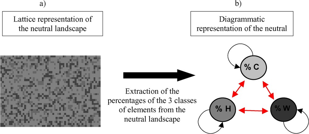
Lattice (a) and diagrammatic (b) representation of a neutral landscape by using three classes of elements: C for crops, H for the hedgerows, and W for wood. The three classes of elements are supposed to be randomly distributed. Arrows represent the individuals that move between the three types of elements and those that stay in the elements.

2.2.2 The population dynamics model

2.2.2.1 The demographic sub-model.

We use a 12-month time unit for the Leslie-type model [31,32]. Thus, A. parallelepipedus life span is divided into three stage classes: larval instars (L) and 2 adult stages (A₁: non-breeders, and A₂: breeders). The demographic parameters (fecundity and survival rates) are defined for this time step. In the landscape, only adults disperse. Sex ratio is on average 1:1 [15]. A. parallelepipedus life cycle is represented by Fig. 2.

Fig. 2
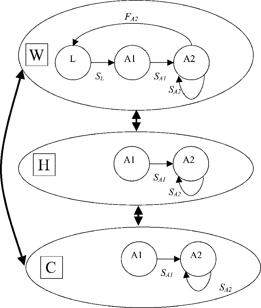
Life cycle of A. parallelepipedus in W, H and C. Bold arrows indicate movements between elements. But for the clearness of the diagram, we did not specify the parameters and stages concerned with movement.

f is fertility. As birth is a flow from April to October, f is defined as a function of the number of eggs laid by one female each year, the survival rate from the egg stage to the larval stage and the A₂ survival rate [33]. Based on experimental data [15,29], we set $f = 2.81$ in W and $f = 0$ in H and C.

$s_{j}^{i}$ is the survival rate. It is defined as the proportion of individuals belonging to the age class j which survive from age j to age $j + 1$ in element i, where $j \in {L, A_{1}, A_{2}}$ and $i \in {W, H, C}$ . The survival rates used in the model are summarized in Table 1. Those for W were taken from [15], those for H from [23]. For C, we used survival rates in cornfield from [23,30]; they are extremely low compared to other habitats. We assumed all survival rates to be density independent.

	Habitats	Stages
		L₁	A₁	A₂
Fecundity	C	0	0	0
	H	0	0	0
	W	0	0	2.81

Survival	C	0	0.05	0.05
	H	0.5	0.45	0.45
	W	0.5	0.45	0.45

Let L be the Leslie block matrix of the demographic model. Because L integrates all demographic parameters for each stage in each element, the dimension of the model is ( $7 \times 7$ ), and L is primitive and is defined as follows:

L = (\begin{matrix} 0 & 0 & F_{A_{2}} \\ S_{L} & 0 & 0 \\ 0 & S_{A_{1}} & S_{A_{2}} \end{matrix})

(1)

with

F_{A_{2}} = f = 2.81

a scalar defining fecundity in W,

S_{j} = s_{j}^{W}

for

j = L

and

S_{j} = diag {s_{j}^{W}, s_{j}^{H}, s_{j}^{C}}

defined as the block matrices of survivals for stage

j \in {A_{1}, A_{2}}

.

2.2.2.2 The movement sub-model.

$d_{i k}$ represents the proportion of individuals present in element of type k and moving toward the element of type i, $0 ⩽ d_{i k} ⩽ 1$ . According to the diagrammatic landscape model (Fig. 1), the movement process may be represented here as a combination of two processes. First, the movement within an element right up to its boundary: we suppose that between two time steps t and $t + Δ t$ , an individual being in element k at time t and moving randomly within this element meets a boundary between k and i with probability p. We also assume that this probability does not depend on element size. If the element i is abundant, an individual moving randomly in the landscape will often encounter it. We thus assume that p only depends on the percentage cover of habitat i ( $p_{i}$ ) in the landscape. Second, boundary behaviour: we denote $q_{i k}$ as the probability of an individual leaving the habitat of type k at the boundary and going towards habitat of type i; $q_{i k}$ is assumed to be independent of the stage j and $0 ⩽ q_{i k} ⩽ 1$ . The coefficients $q_{i k}$ were either measured experimentally [20,25], or estimated by modelling ([30] and non-published data). Their values are given in Table 2. These coefficients show that beetles stay preferentially in suitable habitats (W and H), that they leave C to go towards W, H and that they have the same probability to be in W and H because they are not sensitive to boundaries between woody elements [23]. The proportion of dispersers, $d_{i k}$ , from the habitat k towards habitat i is supposed to be proportional to the parameters q and p, and $d_{i k}$ can be defined as follows:

d_{i k} = q_{i k} p_{i}

(2)

Habitats	W	H	C
W	1	0.5	0.05
H	0.5	1	0.2
C	1	1	1

Let $P = diag {1, P_{A_{1}}, P_{A_{2}}}$ be the dispersal matrix of the dispersal model. 1 is the scalar defining the non-dispersing stage, and $P_{j}$ the matrix block for the dispersing stage with $j \in {A_{1}, A_{2}}$ . $P_{j}$ is defined as follows

P_{j} = (\begin{matrix} 1 - d_{HW} - d_{CW} & d_{WH} & d_{WC} \\ d_{HW} & 1 - d_{WH} - d_{CH} & d_{HC} \\ d_{CW} & d_{CH} & 1 - d_{WC} - d_{HC} \end{matrix})

(3)

2.2.2.3 The spatial Leslie-type model.

We use a classical multiregional Leslie model describing the A. parallelepipedus population dynamics. This type of model is represented as follows:

{\vec{n}}_{t + 1} = LP {\vec{n}}_{t}

(4)

where

{\vec{n}}_{j, t}^{i} = {({\vec{n}}_{L, t}, \dots, {\vec{n}}_{A_{1}, t})}^{T}

is a 7-dimensional ‘element-vector’ giving the number of individuals of age j on habitat i at time t (

j \in {L, A_{1}, A_{2}}

,

i \in {W, H, C}

) and T indicates transposition. The characteristic of the S matrix is the cross classification of individuals by age-class and class of element. The LP matrix entries give the probability that an individual in a given age class and element class becomes or contributes to another age class and element class by the next census. The LP matrix is primitive.

2.2.3 The habitat fragmentation model based on a hierarchical approach of demography and movement

We model habitat fragmentation as a landscape-scale process involving both habitat loss and the breaking apart of habitat (i.e. habitat fragmentation per se) [4]. W loss is measured with the $p_{i}$ -parameter in Eq. (2). Second, we consider in the model not only breaking apart of W but also breaking apart of all types of elements in the landscape. This process increases the probability that an individual encounters a boundary between two elements, and so increases the movement frequency between adjacent elements. For an individual, let k define the number of transition from an element to another for one demographic time unit (1 year). To distinguish between these two time scales, it has been proposed a modification of Eq. (4) [34]:

{\vec{n}}_{t + 1} = {LP}^{k} {\vec{n}}_{t}

(5)

The model allows adjusting dispersal frequency between adjacent patches of elements. k is applied on all elements, but because habitat fragmentation per se is a landscape scale process [4], k can also represent a measure of the ‘W-fragmentation per se’. The more the k-value increases, the more important is the W-fragmentation per se. The combination of these two sub-processes, governed by the k- and $p_{i}$ -parameters, leads to a good approximation of the relationship between the degree of W-fragmentation and the demographic response at the landscape scale.

This implicit modelling approach suggests a particular case of the spatial structure, where the different elements are randomly distributed on the lattice (see Fig. 2). However, due to human pressure, agrosystems are not randomly structured, and H's are linear elements. This representation assumes that every patch of element interacts equally with every other patch of element, i.e. the explicit arrangement of patches, has no effect on the results, and that such models tell us nothing about how the spatial arrangement of habitat destruction affects a population. However, considering in a first attempt H and the agricultural landscape as random structures can be very useful to focus on the role of the element quality and boundaries. Our model can be thus defined as a ‘H₀-hypothesis’ that can be compared to other models where the spatial structure is explicitly integrated (see [35] for a similar example).

2.2.4 Analyses of the model

Construction and analysis of the model was performed with Maple 7^® [36]. The model can be analytically processed through population-level endpoints of the matrix ${LP}^{k}$ : the dominant eigenvalue of the matrix, λ is an estimate of the overall asymptotic population growth rate [33]. We also investigate elasticity analysis (Eq. (2)) to know to which parameter the asymptotic population growth rate is relatively the most sensitive:

e_{i j} = \frac{a_{i j}}{λ} \frac{\partial λ}{\partial a_{i j}} = \frac{\partial \log λ}{\partial \log a_{i j}}

(6)

The concept of demographic elasticity is useful to determine the proportional contribution of matrix elements to the long-term population growth [37]. Values of the elasticity matrix E_a, $e_{i j}$ , are the proportional effects on the population growth rate to proportional changes in each value of the ${LP}^{k}$ matrix. These elasticities sum to 1 across E_a and they can be summed in subsets with respect to elements, stages, element boundaries, or stage transition [38]. We introduce two relative contributions to population growth rate: the proportional perturbation summed within element-classes (‘the element elasticity’) and summed within different boundaries between two classes of elements (‘the boundary elasticity’). It gives the importance of life history events within one element class or boundary between two elements compared overall to life history events in another element class or junction between elements. For example, an important ‘W-elasticity’ (wood elasticity) means that a little increase of W quality (i.e. a little increase of the value of life history rates in W) will increase population viability. We investigate the model through these matrix tools according to W-fragmentation, e.g., decreasing the proportion of W, which we assumed to be replaced by C ( $p_{j}$ -parameter), and increasing the isolation of landscape elements (k-parameter). We build first a pilot study that just includes W and C. We then compare this study with another one with 5% of H. The second one takes into account H, so the comparison of these two studies must give some information on the importance of H and boundaries between H, W and M on the population viability, and their evolution according to W-fragmentation.

3 Results and discussion

The pilot study shows that fragmentation has a negative impact on the asymptotic population growth rate (Fig. 3a). Distinction between habitat loss and habitat fragmentation per se shows that if woodlots cover more than 33% of a landscape, habitat fragmentation has no significant effect: the population is viable and the sensitivity of λ (tangent of the eigenvalue curve) to W-fragmentation is not important. Below 33% of W, effect of habitat loss on population viability depends on the degree of habitat fragmentation per se and sensitivity of λ to W-fragmentation increases exponentially when W-fragmentation per se increases (i.e. population viability decreases exponentially). In the same way, Andrén [39,40] with a model of percolation showed that below a critical threshold of 20% of habitat in a landscape, the isolation distances between patches of habitat will increases exponentially. It also showed for birds and small mammals that when the proportion of suitable habitat is less than 10–30%, the effects of patch area and isolation became greater than expected from habitat loss one. In the elasticity analysis, we show that W are the most important for A. parallelepipedus (maximal elasticity in W: Fig. 4a) and that boundary elasticity (i.e. W/C-elasticity) and C-elasticity can be neglected (quasi null).

Fig. 3
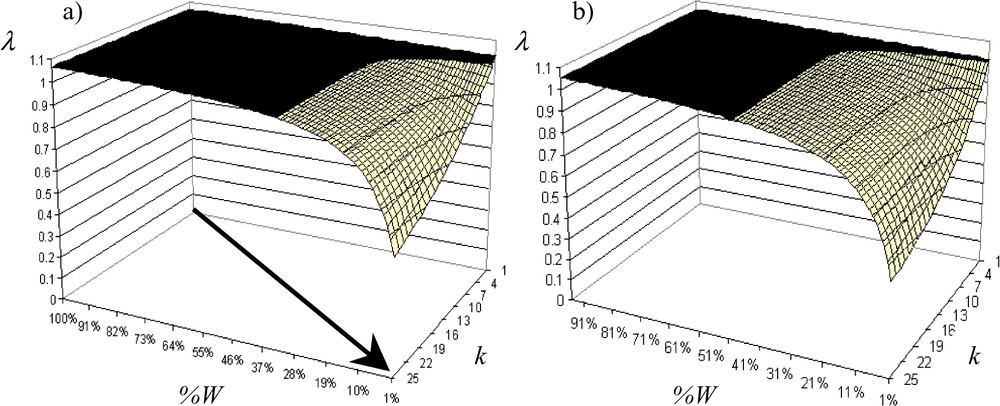
Evolution of the asymptotic population growth rate according to the W fragmentation (■ λ>1: population increases, □ λ<1: population extinction): (a) without H, (b) with 20% of H.

Fig. 4
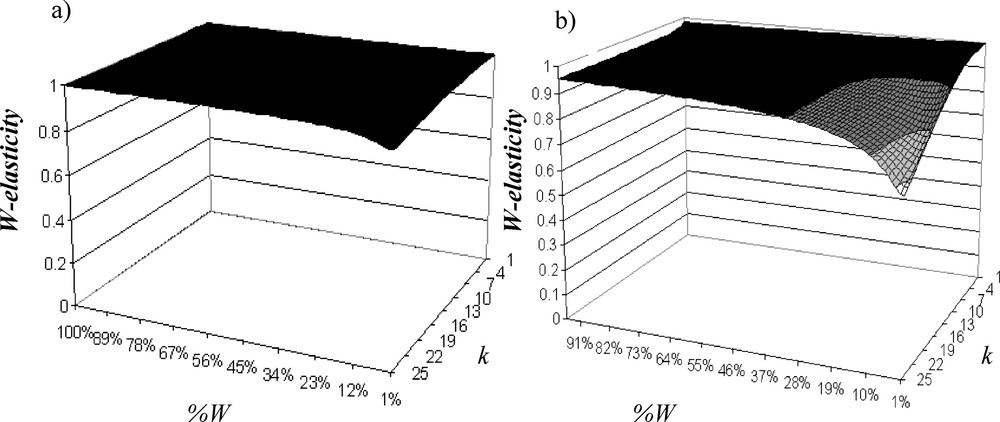
Evolution of the W-elasticity (a) without H, (b) with 20% of H according to the W fragmentation.

The addition of H decreases λ, and the more W fragmentation is important, the more λ decreases (Fig. 3b). Critical threshold of W-loss is increased to 44% of W when W fragmentation per se is a little bit important. Therefore, effect of W fragmentation per se on population viability is weak relative to W loss effect. In fact, when W fragmentation increases, contribution of H (H-elasticity: Fig. 5a) and W/H boundary (W/H-elasticity: Fig. 5b) increases while W-elasticity decreases (Fig. 4b). Contribution of W/H boundary is always important; it increases according to W fragmentation and is very sensitive to W fragmentation per se, while H weight is at maximum 5% of the total elasticity and also depends on W fragmentation. Contributions of C-elasticity and H/C-elasticity are not proportionally important. Elasticity analysis shows that W is the most important element, but when there are H and when fragmentation increases, boundaries between W and H affect the most population viability. Therefore, managing junctions between W and H will determine the population persistence.

Fig. 5
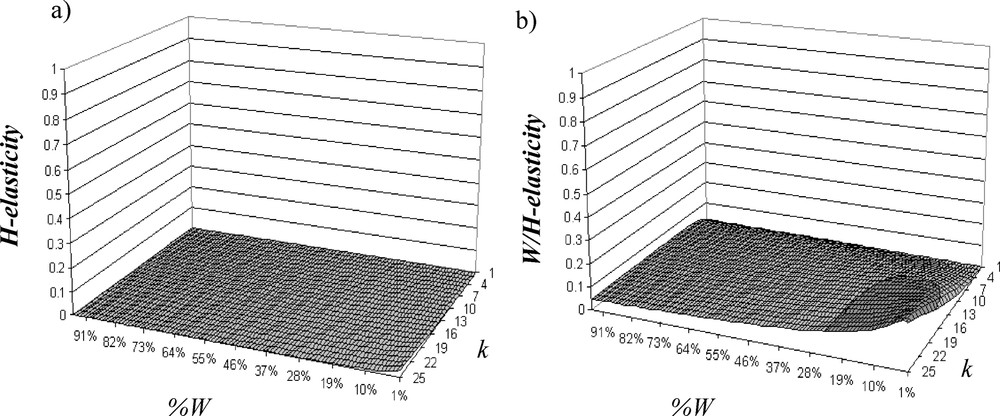
Evolution of (a) H-elasticity and (b) W/H-elasticity (boundary elasticity between W and H), with 20% of H according to the W fragmentation.

For a management point of view, we assume that, even if there are H, when there are few W (for example, 8% on average in Brittany), we must build a single large instead of several small patches of W (i.e., the k-value must be low) to maintain the A. parallelepipedus population at the landscape scale (Fig. 3a and b). The SLOSS debate is an old one and maybe not closed. However, with our model we show in addition to the preceding studies that a single large patch of W increases the proportional sensitivity (elasticity) of the population viability to this single large patch, and decreases the contribution of H, C and boundaries at the landscape scale. Therefore, with a single large patch of W, the spatial context around this single large patch affects less population demography in W and at the landscape scale: the population dynamics at the landscape scale can thus be summarized only by the population dynamics in the single large patch of W.

Models are simplification of the real world: they can be used for different modelling approaches and they are better designed for some particular cases. Our model is better designed for organisms that are not totally specialist or totally generalist (i.e. the quasi-totality of the species) and that evolved in ‘natural’ landscapes where elements are ‘randomly distributed’ (even if, due to natural gradient and pressures, a perfect random distribution of the elements in the landscape is never reached). However, as it has been presented in this paper, this model can be defined as a H₀-hypothesis for spatial structure, and we assume that it is a very useful tool for three other applications:

First, to know which type of approach (the non-spatial, the spatial approach with or without explanation of the landscape matrix) must be applied for the conservation of A. parallelepipedus: there are a lot of models of population dynamics whose reliability has been discussed particularly concerning paucity of data [41–43], need of age structure [41] or importance to adapt modelling to species movement [44], etc. Here, we show that modelling effort (i.e. the number of variables) must be fitted according to the importance of spatial process: a spatial approach is not always required. For example, when there are only W and C and when $W > 33 %$ , the λ-value of our model is not very different from the λ-value in W ( $λ = 1.06$ ) and sensitivity of λ to W-fragmentation is quasi null. Second, spatial data do not need always to be explicit. For example, a simple metapopulation approach (between woodlots) can be used if overall sensitivity of λ to W fragmentation and ‘W elasticities’ are the most important: a metapopulation model for A. parallelepipedus, where the sub-populations are those from woodlots in the landscape, implicitly makes the same assumption. Third, if elasticity of elements between suitable habitats (here H and C) and ‘boundary-elasticity’ are important, elements and boundaries in the landscape matrix between subpopulations must be explicitly incorporated in a population model (as grid-cells models).

Second, to know the degree of specificity of this species: How much habitat fragmentation will affect a species depends on the degree of habitat specialisation of the species [45]. A strict specialist species is absent of all elements except its suitable element. On the other hand, strict generalist species are not sensitive to the variation of landscape structure, and may be found in same densities in all elements of the landscapes. These two extreme positions are not representative of most species that are intermediate. We think that there is a gradient between generalists and specialists, and it is often hard to define the level of specificity for a given species. Our model is a way to compare quantitatively the level of specificity of a species: like comparative analysis of elasticity patterns to stasis [46], it can be useful to compare different types of species via ‘boundary-elasticity’ or ‘elements-elasticity’ patterns (if life history traits are available).

Finally, to study evolutionary demography at the landscape scale: assuming that data on variation and co-variation of life history traits are available, this tool can be a very useful for evolutionary ecology. Using elasticity analysis (‘element-elasticity’ and ‘boundary-elasticity’) in a stochastic way [47–49] is very interesting to know, according to habitat fragmentation, which type of element or boundary minimize or maximize the temporal variation in fitness [50].

4 Conclusion

Our model has important implications for biological conservation in heterogeneous landscapes. It allows assessing the relationship between the degree of habitat fragmentation and the population response at the landscape scale. Because it also distinguishes habitat loss and breaking apart of habitat, we can reply to important questions for conservation biology, “how much habitat is enough?” or for a given proportion of habitat, what kind of spatial management must be maintained for “a single large or several small” patches of habitat? With the elasticity analysis, we can go further in interpretation and know which type of elements and boundaries of the landscape influence the most population viability. However, because our implicit population model does not take into account real spatial arrangement of habitat destruction, we suggest that this model must be used as a first approach to assess the impact of fragmentation on population dynamics. After, it would be important to work on a spatial explicit way, if and only if data are available. However, we lay stress on the importance to use, before using complex explicit models, simple models with few variables that can capture and analyse in a reliable way general landscape patterns.

Acknowledgement

Thanks to Manu Plantegenest and Pavel Kindlmann for their useful comments on the study.

Bibliographie

[1] R.T. Forman; M. Godron Landscape Ecology, John Wiley and Sons, 1986

[2] M.E. Soulé Viable Population for Conservation, Cambridge University Press, New York, 1987

[3] F. Burel; J. Baudry Landscape Ecology: Concepts, Methods, Applications, Science Publishers Inc., New Hampshire, USA, 2003

[4] L. Fahrig Effects of habitat fragmentation on biodiversity, Annu. Rev. Ecol. Evol. Syst., Volume 34 (2003), pp. 487-515

[5] A. Farina Principles and Methods in Landscape Ecology, Chapman & Hall, London, 1998

[6] J.A. Wiens Metapopulation dynamics and landscape ecology (I. Hanski; M. Gilpin, eds.), Metapopulation Biology: Ecology, Genetics and Evolution, Academic Press, San Diego, 1997, pp. 43-62

[7] J.B. Dunning; D.J. Stewart; B.J. Danielson; B.R. Noon; T.L. Root; R.H. Lamberson; E.E. Stevens Spatially explicit population models: current forms and future uses, Ecol. Appl., Volume 5 (1995), pp. 3-11

[8] D.F. Doak; P.C. Marino; P.M. Kareiva Spatial scale mediates the influence of habitat fragmentation on dispersal success: implications for conservation, Theor. Popul Biol., Volume 41 (1992), pp. 315-336

[9] K. McKelvey; B.R. Noon; R.H. Lamberson Conservation planning for species occupying fragments landscapes: the case of northern spotted owl (P.M. Kareiva; J.L. Kingsolver; R.B. Huey, eds.), Biotic Interactions, Global Change, Sinauer Associates, Sunderland, MA, 1993, pp. 424-450

[10] J. Bascompte; R.V. Sole Habitat fragmentation and extinction thresholds in spatially explicit models, J. Anim. Ecol., Volume 65 (1996), pp. 465-473

[11] E.D. McCoy The application of island-biogeographic theory to patches of habitat: how much land is enough?, Biol. Conserv., Volume 25 (1983), pp. 53-62

[12] D. Simberloff The contribution of population and community biology to conservation science, Annu. Rev. Ecol. Syst., Volume 19 (1988), pp. 473-511

[13] F. Burel Landscape structure effects on carabid beetles spatial patterns in western France, Landscape Ecol., Volume 2 (1989), pp. 215-226

[14] S. Petit; F. Burel Connectivity in fragmented populations: Abax parallelepipedus in a hedgerow network landscape, C. R. Acad. Sci. Paris, Ser. III, Volume 321 (1998), pp. 55-61

[15] K. Chaabane; M. Loreau; G. Josens Individual and population energy budgets of Abax ater (Coleoptera, Carabidae), Ann. Zool. Fennici, Volume 33 (1996), pp. 97-108

[16] C.H. Lindroth, 1961–1969. The ground-beetles (Carabidae, excl. Cicindelinae) of Canada and Alaska. Parts 1–6. Opuscula Entomologica xlvii + 1192 pp. 1961, Part 2, Supplementum 20, 1–200; 1963, Part 3, Supplementum 24, 201–408; 1966, Part 4, Supplementum 29, 409–648; 1968, Part 5, Supplementum 33, 649–944; 1969, Part 6, Supplementum 34, 945–1192; Part 1, Supplementum 35, i–xlvii

[17] J.R. Spence Success of European Carabid species in western Canada: Preadaptation for synanthropy?, The Role of Ground Beetles in Ecological Environmental Studies, Intercept Ltd., Andover, UK, 1990

[18] A. Buse Habitat selection and grouping of beetles (Coleoptera), Holarct. Ecol., Volume 11 (1988), pp. 241-247

[19] G. du Chatenet Guide des coléoptères d'Europe – Les guides du naturaliste, Delachaux et Niestlé, Paris, 1986

[20] S. Charrier; S. Petit; F. Burel Movement of Abax parallelepipedus (Coleoptera, Carabidae) in woody habitats of hedgerow network landscape: a radio-tracing study, Agr. Ecol. Environ., Volume 61 (1997), pp. 133-144

[21] S. Petit; F. Burel Effects of landscape dynamics on the metapopulation of a ground beetle (Coleoptera Carabidae) in a hedgerow network, Agr. Ecol. Environ., Volume 69 (1998), pp. 243-252

[22] S. Petit; F. Burel Movement of Abax ater (Col. Carabidae): do forest species survive in hedgerow networks, Vie et Milieu, Volume 43 (1993), pp. 119-124

[23] S. Petit Metapopulations dans les réseaux bocagers : analyse spatiale et diffusion, université de Rennes-1, 1994

[24] E. Fournier; M. Loreau Respective roles of recent hedges and forest patch remnants in the maintenance of ground-beetle (Coleoptera: Carabidae) diversity in an agricultural landscape, Landscape Ecol., Volume 16 (2001), pp. 17-32

[25] M. Martin; F. Bastardie; D. Richard; F. Burel Studying boundary effects on animal movement in heterogeneous landscapes: the case of Abax ater (Coleoptera: Carabidae) in hedgerow network landscapes, C. R. Acad. Sci. Paris, Ser. III, Volume 324 (2001), pp. 1029-1035

[26] M. Loreau Competition in a carabid beetle community: a field experiment, Oikos, Volume 58 (1990), pp. 25-38

[27] P. Greenslade On the ecology of some British beetle with some special reference to life history, Trans. Soc. Br. Entomol., Volume 16 (1965), pp. 149-179

[28] M. Loreau Annual activity and life cycle of two carabid beetles in two forest communities, Holarctic Ecol., Volume 8 (1985), pp. 228-235

[29] K. Chaabane; M. Loreau; G. Josens Growth and egg production in Abax ater (Coleoptera, Carabidae), Pedobiology, Volume 41 (1997), pp. 385-396

[30] L. Tischendorf; U. Irmler; R. Hingst A simulation experiment on the potential of hedgerows as movement corridors for forest carabids, Ecol. Model., Volume 106 (1998), pp. 107-118

[31] A. Rogers Introduction to Multiregional Mathematical Demography, Wiley, New York, 1975

[32] J.-D. Lebreton; G. Gonzalès-Dàvila An introduction to models of subdivided populations, J. Biol. Syst., Volume 1 (1993), pp. 389-423

[33] H. Caswell Matrix Population Models, Sinauer Associates Inc., Sunderland, MA, 2001

[34] E. Sanchez; R. Bravo de la Parra; P. Auger Linear models with different time scales, Acta Biotheor., Volume 43 (1995), pp. 465-479

[35] M.F. Hill; H. Caswell Habitat fragmentation and extinction thresholds on fractal landscapes, Ecol. Lett., Volume 2 (1999), pp. 121-127

[36] K.M. Heal; M.L. Hansen; K.M. Rickard Maple 7^®, Waterloo Maple Inc., Waterloo, Canada, 2001

[37] H. de Kroon; A. Plaisier; J. van Groenendael; H. Caswell Elasticity: the relative contribution of demographic parameters to population growth rate, Ecology, Volume 67 (1986), pp. 1427-1431

[38] J.B. Pascarella; C.C. Horvitz Hurricane disturbance and the population dynamics of a tropical understory shrub: megamatrix analysis, Ecology, Volume 79 (1998), pp. 547-563

[39] H. Andrén Effects of habitat fragmentation on birds and mammals in landscapes with different proportions of suitable habitat: a review, Oikos, Volume 71 (1994), pp. 355-366

[40] H. Andrén Habitat fragmentation, the random sample hypothesis and critical thresholds, Oikos, Volume 84 (1999), pp. 306-308

[41] U. Wennergren; M. Ruckelshaus; P. Kareiva The promise and limitations of spatial models in conservation biology, Oikos, Volume 74 (1995), pp. 349-356

[42] M. Ruckelshaus; C. Hartway; P. Kareiva Assessing the data requirements of spatially explicit dispersal models, Conserv. Biol., Volume 11 (1997), pp. 1298-1306

[43] A. South Dispersal in spatially explicit population models, Conserv. Biol., Volume 13 (1999), pp. 1039-1046

[44] A.B. South; S.P. Rushton; R.E. Kenward; D.W. Macdonald Modeling vertebrate dispersal and demography in real landscapes: how does uncertainty regarding dispersal behaviour influence predictions of spatial population dynamics? (J. Bullock; R. Kenward; R. Hails, eds.), Dispersal Ecology, Blackwell Science Ltd., London, 2001

[45] H. Andrén Habitat fragmentation and changes in biological diversity, Ecol. Bull., Volume 46 (1997), pp. 171-181

[46] L.B. Crowder; D.T. Crouse; S.S. Heppell; T.H. Martin Predicting the impact of turtle excluder devices on loggerhead sea turtle populations, Ecol. Appl., Volume 4 (1994), pp. 437-445

[47] T.G. Benton; A. Grant Elasticity analysis as an important tool in evolutionary and population ecology, Trends Ecol. Evol., Volume 14 (1999), pp. 467-471

[48] T.G. Benton; A. Grant How to keep fit in the real world: elasticity analyses and selection pressures on life-histories in a variable environment, Am. Nat., Volume 147 (1996), pp. 115-139

[49] S. Tuljapurkar; C.C. Horvitz; J.B. Pascarella The many growth rates and elasticities of populations in random environments, Am. Nat., Volume 162 (2003), pp. 489-503

[50] C. Pfister Patterns of variance in stage-structured populations: evolutionary predictions and ecological implications, Proc. Natl Acad. Sci. USA, Volume 95 (1998), pp. 213-218

Commentaires - Politique