ISSCOR: Intragenic, Stochastic Synonymous Codon Occurrence Replacement – a new method for an alignment-free genome sequence analysis

Jan P. Radomski; Piotr P. Slonimski

doi:10.1016/j.crvi.2008.11.008

Genetics / Génétique

ISSCOR: Intragenic, Stochastic Synonymous Codon Occurrence Replacement – a new method for an alignment-free genome sequence analysis
[ISSCOR : une nouvelle méthode pour une analyse des séquences de génome sans alignement]

Présenté par : Jean Rosa

Jan P. Radomski ¹ ; Piotr P. Slonimski ²

¹ Interdisciplinary Center for Mathematical and Computational Modeling, Warsaw University, Pawińskiego 5A, Bldg. D, 02106 Warsaw, Poland
² Centre de génétique moléculaire du CNRS & Université Pierre-et-Marie Curie (Paris-6), 91190 Gif-sur-Yvette cedex, France

Comptes Rendus. Biologies, Volume 332 (2009) no. 4, pp. 336-350.

Résumés

Anglais
Français

Synonymous codons do not occur at equal frequencies. Codon usage and codon bias have been extensively studied. However, the sequential order in which synonymous codons appear within a gene has not been studied until now. Here we describe an in silico method, which is the first attempt to tackle this problem: to what extent this sequential order is unique, and to what extent the succession of synonymous codons is important. This method, which we called Intragenic, Stochastic Synonymous Codon Occurrence Replacement (ISSCOR), generates, by a Monte Carlo approach, a set of genes which code for the same amino acid sequence, and display the same codon usage, but have random permutations of the synonymous codons, and therefore different sequential codon orders from the original gene. We analyze the complete genome of the bacterium Helicobacter pylori (containing 1574 protein coding genes), and show by various, alignment-free computational methods (e.g., frequency distribution of codon-pairs, as well as that of nucleotide bigrams in codon-pairs), that: (i) not only the succession of adjacent synonymous codons is far from random, but also, which is totally unexpected, the occurrences of non-adjacent synonymous codon-pairs are highly constrained, at strikingly long distances of dozens of nucleotides; (ii) the statistical deviations from the random synonymous codon order are overwhelming; and (iii) the pattern of nucleotide bigrams in codon-pairs can be used in a novel way for characterizing and comparing genes and genomes. Our results demonstrate that the sequential order of synonymous codons within a gene must be under a strong selective pressure, which is superimposed on the classical codon usage. This new dimension can be measured by the ISSCOR method, which is simple, robust, and should be useful for comparative and functional genomics.

Les codons synonymes n'apparaissent pas à des fréquences égales. L'usage des codons et le biais codonique ont été abondamment étudiés. Par contre, l'ordre dans lequel les codons synonymes se présentent le long d'un gène n'a pas encore été analysé. Cet ordre est-il unique ? A quel point l'enchaînement des codons synonymes non-adjacents est-il important ? Nous présentons ici une nouvelle méthode in silico pour aborder ce problème. Dans cette méthode, appelée ISSCOR, on permute, par une approche Monte-Carlo, les codons synonymes d'un gène. On obtient ainsi un ensemble de séquences nucléotidiques, qui ont le même usage des codons, qui codent pour la même séquence protéique, mais qui diffèrent par l'ordre des codons synonymes. Nous avons analysé la totalité du génome de la bactérie Helicobacter pylori (1574 ORFs) et nous démontrons, par différentes approches informatiques (analyse de la fréquence de distribution des paires de codons ainsi que celle des bigrams de nucléotides dans des paires de codons), que : (i) les codons synonymes s'enchaînent dans un ordre déterminé sur de longues distances (douzaines de nucléotides) ; (ii) l'enchaînement des codons synonymes le long d'un gène est en relation directe avec le codage de la protéine ; (iii) les bigrams nucléotidiques situés sur des paires de codons peuvent être utilisés comme une nouvelle méthode, simple et robuste, pour caractériser les gènes et les génomes.

Métadonnées

Reçu le : 2008-11-11
Accepté le : 2008-12-02
Publié le : 2009-02-03

PMID

DOI : 10.1016/j.crvi.2008.11.008

Keywords: Alignment free analysis, Random codon shuffling, Sequential order of synonymous codons, Synonymous codon replacement
Mots-clés : Analyse sans alignement, Réarrangement aléatoire des codons, Ordre séquentiel de codons synonymes, Remplacement de codons synonymes

Affiliations des auteurs :

Jan P. Radomski ¹ ; Piotr P. Slonimski ²

¹ Interdisciplinary Center for Mathematical and Computational Modeling, Warsaw University, Pawińskiego 5A, Bldg. D, 02106 Warsaw, Poland
² Centre de génétique moléculaire du CNRS & Université Pierre-et-Marie Curie (Paris-6), 91190 Gif-sur-Yvette cedex, France

@article{CRBIOL_2009__332_4_336_0,
     author = {Jan P. Radomski and Piotr P. Slonimski},
     title = {ISSCOR: {Intragenic,} {Stochastic} {Synonymous} {Codon} {Occurrence} {Replacement} {\textendash} a new method for an alignment-free genome sequence analysis},
     journal = {Comptes Rendus. Biologies},
     pages = {336--350},
     publisher = {Elsevier},
     volume = {332},
     number = {4},
     year = {2009},
     doi = {10.1016/j.crvi.2008.11.008},
     language = {en},
}

TY  - JOUR
AU  - Jan P. Radomski
AU  - Piotr P. Slonimski
TI  - ISSCOR: Intragenic, Stochastic Synonymous Codon Occurrence Replacement – a new method for an alignment-free genome sequence analysis
JO  - Comptes Rendus. Biologies
PY  - 2009
SP  - 336
EP  - 350
VL  - 332
IS  - 4
PB  - Elsevier
DO  - 10.1016/j.crvi.2008.11.008
LA  - en
ID  - CRBIOL_2009__332_4_336_0
ER  -

%0 Journal Article
%A Jan P. Radomski
%A Piotr P. Slonimski
%T ISSCOR: Intragenic, Stochastic Synonymous Codon Occurrence Replacement – a new method for an alignment-free genome sequence analysis
%J Comptes Rendus. Biologies
%D 2009
%P 336-350
%V 332
%N 4
%I Elsevier
%R 10.1016/j.crvi.2008.11.008
%G en
%F CRBIOL_2009__332_4_336_0

Jan P. Radomski; Piotr P. Slonimski. ISSCOR: Intragenic, Stochastic Synonymous Codon Occurrence Replacement – a new method for an alignment-free genome sequence analysis. Comptes Rendus. Biologies, Volume 332 (2009) no. 4, pp. 336-350. doi : 10.1016/j.crvi.2008.11.008. https://comptes-rendus.academie-sciences.fr/biologies/articles/10.1016/j.crvi.2008.11.008/

Version originale du texte intégral

1 Introduction

The genetic code is degenerate. The relative frequency with which synonymous codons are used may vary widely from species to species, or from one gene (or a class of genes) to another. A large, and ongoing, body of literature deals with this subject under various headings, such as “codon usage”, “codon bias”, “codon adaptation”, etc. [1–17].

It is of significant interest to ask if, and to what extent, the genetic, molecular and cellular apparatus of each species is geared towards actual codon patterns of each sequence in the genome during translation and protein expression. The first part is obviously rhetorical, as there are plenty of indicators that such differences are not only present, but in fact crucial, and influence the steady state ratio of various proteins. Living organisms have very often quite biased preferences for some synonymous codons over other possible synonymous nucleotide triplets coding for the same amino acids. These differences and their variation have been extensively studied, however, no decisive governing rules have yet been discovered. Frequencies of codons for many species are in close correlation with their genome's GC contents, but the underlying forces governing this are not clear – it might be possible, that it is the GC content which is determining a genome's amino acids predilection for the specific codons being used and their bias. On the other hand it might be that reverse causative relationships are in operation: codons-specific amino acids usage is a driving factor for observed GC contents. Possible factors and forces driving synonymous codons usage postulated so far include, among many others: translational optimization [2–6], mRNA structural effects [7], protein composition [8], and protein structure [9], gene expression levels [2,10], the tRNA abundance differences between different genomes, and tRNA optimization [11–13], different mutation rates and patterns [14]. Also, some other possibilities were hypothesized, like local compositional bias [15], and even gene lengths might play a role too [16].

It is clear, that many interesting biological mechanisms underlie the basic phenomenon of genetic code degeneracy. One of its aspects, however, has not been studied until now, namely, the question dealing with the sequential order of occurrence of synonymous codons. To what extent this order is characteristic for a gene, to what extent for a set of genes, or a genome. Are there some rules governing such an order? How can one measure the order of synonymous codons, and compare different orders? Obviously, an order of elements in a linear set is a different property, than the frequency of elements in the set. The amino acid composition of a protein (which formally is exactly equivalent to the synonymous codon frequency, or codon usage, of a protein coding sequences) carries much less information than the amino acid sequence of such protein, which in turn is less information intensive than a corresponding nucleotide sequence coding the same protein.

This question can be formulated more precisely. Let us consider a given frequency of synonymous codon usage characteristic for a gene. There is a very large number of different orders in which the synonymous codons can appear sequentially along the gene without changing either the amino acid sequence of the encoded protein, or the codon usage of the gene. For all practical purposes this number is infinite, since the number of permutations of synonymous codons in a gene is comparable to the number of permutations of amino acids in a protein.

However, there are few means available experimentally to actually attempt even simplest direct measurements of the factors involved. Here, we describe an in silico method, which, as far as we know, is the first attempt to tackle the problem of the sequential order of synonymous codons. We call it ISSCOR (Intragenic, Stochastic Synonymous Codon Occurrence Replacement) for following reasons: (i) it analyses a original single gene, the nucleotide sequences of an original protein coding sequence (ORF). Of course, after analyzing several individual genes, the results can be computed for a set of genes, or a complete genome; (ii) it is essentially a Monte-Carlo approach. Synonymous codons, which occur at different positions of an ORF are replaced randomly, with the frequencies given by the codon usage of the whole genome. The method generates nucleotide sequences of non-original ORFs, which have identical codon usages, and would encode identical amino acid sequences. It is equivalent to random permutations of the synonymous codon sequence.

We have chosen to test the application of the ISSCOR method on the genome of Helicobacter pylori. This organism was selected for two reasons: (i) the H. pylori codon usage is not dominated by biased mutation patterns and displays a striking absence for transitionally mediated selection among synonymous codons [17]; and (ii) the H. pylori genome shows a striking periodic oscillations of it's nucleotide sequence, and it was hypothesized that these oscillations could be related to the usage of particular synonymous codons for constructing α-helical protein folds [18]. To this end we have retrieved (as of October 2006) from TIGR the complete set of H. pylori protein coding sequences, however, due to the needs of the ISSCOR algorithms, only those containing unambiguously assigned nucleotides (A, C, G, and T, in standard notation) have been used – this resulted in 1574 ORFs.

2 The concepts and methods used

2.1 The concept of Intragenic, Stochastic Synonymous Codon Occurrence Replacement

For the reasons outlined briefly above in the Introduction, we describe here the method of calculating the whole genome codon-pair pattern profiles, as well as assessing their significance. Previously [18–21] we have described alignment free approaches to the problem of comparison and analysis of complete genomes, and some techniques enabling us to cope with the sparseness of the n-gram type of genomic information representations. The problem of sparse occurrence matrices is not only present, but even more pronounced when dealing with the number of permutations of the possible synonymous codons. Calculating the set of n-grams for such occurrences will lead to a vector representation, which is severely sparse, especially for higher n-grams lengths, and hence to very poor statistics. To alleviate this problem, we propose here a hybrid approach. Namely, when computing counts of codon-pair patterns – separated by codon sub-sequences of differing length – the actual composition of these spacer sub-sequences will be neglected. However, when such partial counts are used as a composite set, poor statistics are no longer a hindering obstacle, and the complete information about particular n-gram frequencies profile is preserved, albeit in a distributed and convoluted form.

There are only two requirements fundamental for the ISSCOR method: (a) the amino acid sequence of every protein in the whole genome must be strictly preserved; (b) random shuffling of synonymous codons will be performed separately within each codon-degeneracy equivalence group using uniform probability distribution (thus, the codon usage profile for the whole genome, after the synonymous codon shuffling will be preserved within stochastic bounds of uniform probability distribution, and the overall codon usage of the whole genome will not be changed).

For every protein coding gene, with its original nucleotide sequence $j_{0}$ in a genome i we generate, by a Monte Carlo approach, a set of equivalent nucleotide strings ( $j_{1}, j_{2}, j_{3}, \dots, j_{N}$ ) which have the following properties:

• they have the same nucleotide lengths as the $j_{0}$ ;
• they have the exactly the same amino acid sequence as the $j_{0}$ (i.e., the proteins translated from the $j_{1}, j_{2}, j_{3}, \dots, j_{N}$ are identical);
• they have, on average, the same codon usage frequencies (i.e., the codon triplet occurrence frequency) as the whole genome, and if the gene under study has no codon bias, the same codon usage as $j_{0}$ ;
• they have in the vast majority of cases a synonymous codon order different from the original sequence $j_{0}$ .

This is an essential point, which merits a commentary. The probability that a given string

j_{i}

generated stochastically has the same synonymous codon order as the original

j_{0}

decreases with the product of its length, with a probability limit tending rapidly to zero (e.g., for the gene HP1355, Fig. 1, this probability is less than 10⁻³ for the first six codons, shown in Fig. 1, while the whole gene length is actually 215 codons, thus such probability for this gene is vanishingly small).

Fig. 1
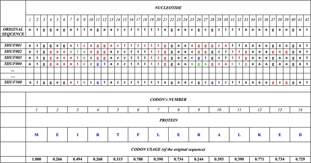
Example of synonymous codon replacements by the ISSCOR method, preserving the amino acid sequence of a gene. The beginning of (the first 14 codons) the original, genuine sequence of the gene HP1355 (coding for the nicotinate–nucleotide phosphorylase) is shown in the first line; the synonymous codons are replaced randomly using the frequencies given in the last line. The first run of replacement's (SHUF001) produces the nucleotide sequence, where synonymous codons, which are different from original are shown in red; in successive runs (SHUF002, 003, 004, until 500), other replacements appear (shown in green and blue). The frequency of occurrence of each of the 144 BiHex patterns (Table 3) is calculated for every run of replacements, i.e., separately for sequences SHUF001,002,…,500; finally the averages, their standard deviations; and deviates are calculated as explained in the text. The amino acid sequences are, of course, identical.

Therefore, the ISSCOR method allows comparing the original codon sequence with an ensemble of different synonymous sequences-coding for the same amino acids sequence.

2.2 The computational procedure

Mathematically speaking, first, the whole genome's codon usage frequencies are determined for each species i, and on that basis probabilities of replacement are calculated separately for each codon-degeneracy equivalence group d:

P_{i}^{k} = \frac{u_{k}}{\sum_{d = 1}^{E} u_{d}}

(1)

where:

P_{i}^{k}

is the probability that any other codon – from the same degeneracy equivalence group d – will be randomly replaced by the codon k; and

u_{k}

is the synonymous codon k triplet frequency for a given amino acid in a whole genome. Therefore, obviously for any given degeneracy equivalence group d, the sum of such probabilities will always be equal to 1.

Then, successively for each codon in a gene the procedure of it's synonymous random replacement is performed based on probabilities according to Eq. (1). Finally, the resulting shuffled sequences are determined, and compared to the original sequence of the gene.

To this end we need, first of all to calculate series of codon-pair pattern¹ occurrence matrices, designed henceforth as $O_{i}^{λ}$ , for the original genome i. The method described here is applicable to any genome, and is independent of the respective genome sizes.

The method involves several steps (although, depending on the actual purpose at hand, not all the chain will be always necessary). For completeness sake, we present them here sequentially, to facilitate understanding.

First, for each protein coding sequence, we determine a complete matrix of all codon-pair patterns. Obviously, in a protein coding gene, there are at most 3904 ( $61 \times 61 + 61 \times 3$ ) unique codon-pair patterns. For a given sequence V, and the all codon-spacer lengths, in order to calculate observed values of a particular codon-pair pattern ( $c_{k}, c_{l}$ ), first we need to construct a series of matrices $O^{λ}$ (occurrence matrices). Each element of every matrix $O^{λ}$ contains the counted sum of all specific codon-pair patterns ( $c_{k}, c_{l}$ ), separated by a string of other codons present in this sequence, where the λ denotes the number of other codons separating the given codon-pair pattern ( $c_{k}, c_{l}$ ). Using a sliding window of the length $3 * (λ + 2)$ nucleotides, and starting at the position m, we would scan the whole sequence V, calculating elements of the matrix by the formula:

O^{λ} (c_{k}, c_{l}, p) = \sum_{m = 1}^{M - λ - 1} f (c_{k}, c_{l}, λ, m, p),

(2)

where M is the sequence's length, and

f (c_{k}, c_{l}, λ, m, p) = {\begin{matrix} 1, & if V (m) = c_{k}, and V (m + λ + 1) = c_{l}, and \\ the codon-pair pattern (c_{k}, c_{l}) matches \\ the pattern of the particular comparison p, \\ 0, & otherwise . \end{matrix}

Comparisons involve matches between the predefined codon-pair patterns, of the first codon $c_{k}$ , taken together with the second codon $c_{l}$ .

That is, a particular positional comparison p involves only one nucleotide from the first codon $c_{k}$ , and one nucleotide from the second codon $c_{l}$ , ignoring all four remaining nucleotides, which corresponds to a BiHex pattern (see footnote 1). Thus, there are, e.g., nine BiHex patterns containing the adenine (A) at any position in a first codon, together with the cytosine (C) at any position in a second codon, etc. Obviously, when $λ = 0$ , one has an adjacent codon-pair pattern (hexanucleotide), for $λ = 1$ it is a nonanucleotide, and so on. Note, that since these are ordered counts, each starting at the sequence's 5′-terminus, the matrices $O_{i}^{λ}$ are not symmetrical, that is the count of the hexon ( $c_{k}, c_{j}$ ) is different from the count of the hexon ( $c_{j}, c_{k}$ ). For each of species i, their hexon counting is repeated for all sequences of the whole genome separately, but the results are then summed up for all sequences, and all respective particular pattern comparisons p. Therefore matrices $O_{i}^{λ}$ should be considered as a raw, spacer λ dependent, representation of sui generis species specific occurrences of their hexons unique patterns.

To make the results independent of a particular genome size (or a subset of genes), we propose to calculate how much the number of actually observed hexons in the original genome, differs from the mean number of the corresponding hexons, observed after performing N random ISSCOR genome permutations, divided by the standard deviation observed in the shuffled genomes:

D_{x A x_λ_T x x} = \frac{O_{occurrences} - \frac{(\sum_{n}^{N} R_{shuffled}^{n})}{N}}{{STD}_{shuffled}}

(3)

where:

$D_{x A x_λ_T x x}$ is a deviate of the results for, e.g., the pattern $x A x_λ_T x x$ , that is for the all codon combinations comprising the nucleotide A at the second position in the first codon, and the nucleotide T at the first position of the second codon – the border codons being separated by the number λ of other codons;
$O_{occurrences}$ are the numbers of the actually observed occurrences for any given hexon in the unperturbed, whole genome;
$R_{shuffled}^{n}$ are the numbers of occurrences for any given hexon pattern counted after codons of the whole genome have been shuffled randomly (as described by the above), thus the $R_{shuffled}^{n} / N$ is a mean number of such occurrences after the N such random shuffles;
${STD}_{shuffled}$ is a standard deviation for all occurrences of a given hexon pattern, after N random shufflings of the whole genome.

We have verified that $N = 500$ is sufficient to ensure satisfactory randomness since the results are practically identical for $N = 500$ , 1000, and 1500.

3 Results and discussion

In order to facilitate the comprehension of the BiHex concept, and that of the first results obtained, we shall begin by an example, the detailed analysis of just one particular BiHex pattern: xxG-xxG for $λ = 6$ . It should be remembered that for all the examined λs there are 4455 ( $135 \times 33 = 4455$ ) different and informative² BiHex patterns, all of which have been computed in this work.

3.1 Detailed description of an example: analysis of just one BiHex pattern “xxG-xxG” for $λ = 6$ demonstrates that specific non-adjacent codon-pairs are strongly constrained in the original protein coding genes

This BiHex pattern, (where the symbol ${}^{○}{BH}_{p = 131}^{λ = 6}$ , or ${BH}_{131}^{6}$ in a shorthand notation, denotes the BiHex of the pattern number 131, and with the codon-spacer $λ = 6$ ) can be written explicitly as xxGyyyyyyyyyyyyyyyyyyxxG. It corresponds to all the oligonucleotides (24 mers; as previously described, the “x” denotes any nucleotide found in the initial and terminal codons of a given BiHex pattern, and the “y” denotes any nucleotide constituting the spacer part between the respective initial and terminal codons of such a BiHex pattern), occurring in the reading frame zero, of the Helicobacter pylori protein coding genes. The analysis comprises several successive steps:

Observed	AAG	ACG	AGG	ATG	CAG	CCG	CGG	CTG	GAG	GCG	GGG	GTG	TAG	TCG	TGG	TTG	Sum
AAG	250	65	109	172	61	28	15	41	224	168	236	292	10	34	65	294	2064
ACG	84	56	45	112	30	22	1	23	79	97	137	131	1	28	32	147	1025
AGG	93	40	61	83	20	17	3	24	86	83	78	127	2	29	38	122	906
ATG	189	96	98	254	76	35	10	50	207	226	224	321	9	46	77	358	2276
CAG	67	26	20	60	22	6	6	22	61	61	60	80	0	12	24	80	607
CCG	33	14	13	41	16	10	4	8	27	36	37	61	1	9	15	60	385
CGG	9	6	4	11	7	3	1	4	12	14	18	20	2	2	3	16	132
CTG	40	21	17	49	7	6	3	10	41	51	59	54	1	11	25	59	454
GAG	228	82	95	154	47	24	12	50	248	178	186	245	5	31	48	231	1864
GCG	201	78	99	218	56	31	15	42	178	275	267	326	7	41	73	331	2238
GGG	205	117	91	220	62	37	17	42	209	290	330	349	4	49	89	338	2449
GTG	298	136	102	310	66	71	12	48	239	326	367	477	9	68	124	444	3097
TCG	43	25	19	47	15	4	0	7	34	34	41	51	2	13	13	69	417
TGG	67	38	32	80	16	16	5	13	53	78	102	111	4	17	37	95	764
TTG	280	146	119	298	87	39	16	78	275	299	361	437	11	63	103	529	3141
Sum	2087	946	924	2109	588	349	120	462	1973	2216	2503	3082	68	453	766	3173	21 819

Averages	AAG	ACG	AGG	ATG	CAG	CCG	CGG	CTG	GAG	GCG	GGG	GTG	TAG	TCG	TGG	TTG	Sum
AAG	240	89	88	159	62	31	11	42	206	189	196	273	9	36	66	288	1985
ACG	94	57	37	102	28	17	5	21	82	106	105	121	3	19	35	143	972
AGG	84	37	42	84	23	13	5	17	77	80	91	114	3	16	34	117	837
ATG	200	103	93	254	59	33	12	54	191	221	240	312	5	45	77	369	2269
CAG	60	26	24	50	20	10	3	11	54	51	51	70	2	11	16	77	536
CCG	31	19	13	35	9	6	2	7	29	31	33	42	1	6	15	49	328
CGG	10	5	5	10	3	2	1	2	10	10	11	14	0	2	4	15	105
CTG	42	19	17	43	11	7	2	10	37	43	44	59	2	9	14	71	430
GAG	221	84	82	139	55	28	10	35	217	172	172	219	6	33	48	238	1759
GCG	191	97	84	222	53	34	11	45	171	224	234	276	6	39	68	305	2059
GGG	182	119	85	219	51	34	11	43	171	250	282	304	5	44	85	292	2177
GTG	256	130	110	272	67	49	14	55	222	285	331	409	9	54	107	378	2749
TCG	36	19	16	42	11	5	2	9	32	40	41	52	1	8	14	61	390
TGG	64	34	29	80	15	12	4	14	53	72	88	103	3	13	37	99	720
TTG	289	129	121	294	74	47	15	71	252	292	306	404	11	58	100	483	2947
Sum	2001	968	846	2005	539	328	107	435	1805	2068	2226	2773	67	392	721	2984	20 264

Fig. 2A
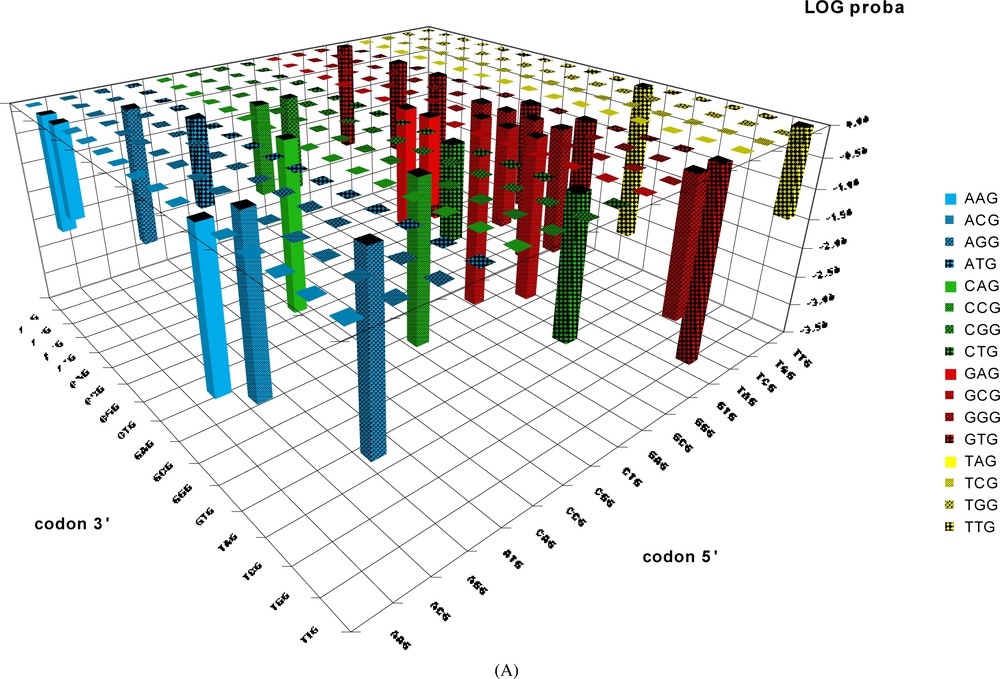
Probability of occurrence by chance of codon-pairs corresponding to the BiHex pattern xxG-λ=6-xxG. The probabilities (shown on a vertical axis in a log. scale) of occurrence by chance of the 240 hexon patterns were calculated from the $χ^{2}$ values given by Table 2C (only the patterns giving probabilities <0.05 are shown). The patterns should be read in the order: codon 5′–codon 3′; thus the probability for the pattern TTGyyyyyyyyyyyyyyyyyyGCG is close to 10⁻³, and that of GTGyyyyyyyyyyyyyyyyyyTTG is close to 10⁻⁴, etc.

Fig. 2B
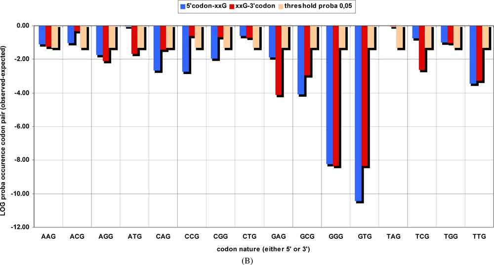
Probability of occurrence by chance of groups of codons pairs, corresponding to the BiHex pattern xxG-λ=6-xxG. The number of occurrences of all hexons beginning (in blue) with the codons given in the abscissa, or those terminated (in red) by them, were summed up for the original genes (Table 2A) and for the permuted ones (Table 2B). The $χ^{2}$ and probabilities were calculated, and the latter are shown on the ordinate in a log scale. Thus, the probability for the GTG-λ=6-xxG pattern is close to 10⁻¹⁰, etc.

Yates Chi²	AAG	ACG	AGG	ATG	CAG	CCG	CGG	CTG	GAG	GCG	GGG	GTG	TAG	TCG	TGG	TTG	Sum
AAG	0.34	6.36	4.77	0.99	0.00	0.27	1.12	0.01	1.56	2.30	8.07	1.27	0.06	0.04	0.01	0.11	3.09
ACG	0.87	0.01	1.75	0.91	0.14	1.00	2.21	0.19	0.06	0.64	9.53	0.69	nc	3.75	0.12	0.10	2.84
AGG	0.97	0.11	7.85	0.00	0.19	1.19	0.70	2.65	0.91	0.10	1.65	1.33	nc	10.11	0.41	0.14	5.63
ATG	0.58	0.46	0.26	0.00	4.37	0.11	0.10	0.21	1.21	0.08	0.98	0.23	nc	0.00	0.00	0.30	0.02
CAG	0.67	0.00	0.63	1.93	0.09	1.00	nc	9.84	0.83	1.66	1.45	1.39	nc	0.06	3.22	0.08	9.33
CCG	0.06	0.98	0.00	0.75	4.62	1.64	nc	0.02	0.11	0.57	0.38	8.68	nc	0.73	0.00	2.37	9.68
CGG	0.08	0.17	0.14	0.00	nc	nc	nc	nc	0.32	1.31	3.21	1.83	nc	nc	nc	0.01	6.43
CTG	0.05	0.14	0.00	0.70	0.96	0.04	nc	0.00	0.30	1.48	4.43	0.33	nc	0.47	7.03	1.81	1.29
GAG	0.17	0.02	1.97	1.46	1.07	0.41	0.21	6.44	4.38	0.16	1.07	2.87	0.01	0.07	0.00	0.17	6.19
GCG	0.44	3.51	2.55	0.04	0.12	0.15	1.26	0.14	0.24	11.53	4.39	9.03	0.03	0.04	0.32	2.15	15.46
GGG	2.83	0.01	0.36	0.00	2.26	0.19	3.20	0.00	7.98	6.28	7.83	6.42	0.12	0.37	0.16	7.22	33.89
GTG	6.76	0.21	0.56	5.25	0.01	9.62	0.14	0.84	1.24	5.61	3.74	11.16	0.02	3.51	2.53	11.18	43.83
TCG	1.32	1.29	0.44	0.38	1.28	0.18	1.14	nc	0.05	0.85	0.00	0.01	nc	3.11	0.04	1.05	1.77
TGG	0.07	0.34	0.25	0.00	0.06	0.86	0.16	nc	0.00	0.36	2.20	0.50	nc	1.20	0.01	0.11	2.62
TTG	0.28	2.17	0.01	0.05	2.26	1.19	0.00	0.67	1.94	0.12	9.78	2.54	0.01	0.28	0.05	4.35	12.69
Sum	3.65	0.48	7.01	5.33	4.37	1.31	1.54	1.63	15.61	10.58	34.37	34.34	0.01	9.18	2.78	11.94	119.27

Contrary to numerous studies on the occurrence and the biases of adjacent codon-pairs [22–27], the analysis of non-adjacent codon-pairs is extremely limited. Only one study deals with this problem [23]. Based upon limited data available at that time (non-complete genome sequences of E. coli, S. cerevisiae, and H. sapiens) Hatfield and Gutman observed that the occurrence of non-adjacent codon-pairs is non random at long distances. Their data were obtained by pooling together all the possible 3904 codon-pairs into one bin only. The authors conclude that “the basis of this effect remains a mystery”. As far as we know, no analysis of this problem has been continued. Here we have shown that the different synonymous codon-pairs, specific for different distances, are responsible for the distant codon-pairs biases.

3.2 Perusal of all the informative 135 BiHex patterns for $λ = 0$ demonstrates, that all six positions of a pair of adjacent codons are constrained

It would be very tedious and undigestable to analyze in depth, in a manner analogous to that shown in Tables 2A–2C, all the 135 BiHex patterns listed in Table 1, for all the spacer codons λ from 0 to 32 (which would represent an equivalent of $135 \times 33 \times 3 = 13 365$ such individual tables!). Furthermore, this is not in the scope of the present article, which aims rather at the description of a novel method in computational biology of genomes. We believe that the introduction of the BiHex notation, both as a concept, and as a new method of computation, will be a successful shorthand for the description of profound and unexpected discoveries of the genuine, original order of synonymous codons whose nature and evolutionary significance remains to be understood. The results shown in Figs. 3A, 3B illustrate this notion.

Fig. 3A
BiHex patterns significantly deviating in the original genome for the adjacent codon-pairs (codon-spacer λ = 0). The number of occurrences of the BiHex patterns for λ = 0 (here, hexons correspond to hexanucleotides) are calculated for the original genome, and compared with their corresponding average number of occurrences in the 500 ISSCOR permutations (Eq. (3)). The difference, between original and the averaged permuted number of occurrences, is expressed in standard deviation units (STD). For clarity, we plot the deviates in two opposite directions – the patterns over-represented in the original above the zero line, and these under-represented below the zero line; with the negative sign. All BiHex patterns shown significantly deviate from randomness, some of them more than 100 STD (e.g., xxT-Txx – over-represented; and xxA-xxT – under-represented).

Fig. 3B
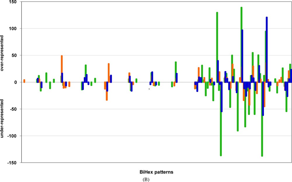
Examples of BiHex patterns significantly deviating in the original genome for the non-adjacent codon-pairs. The order of BiHex patterns, on the abscissa, is the same as in Fig. 3A, but their symbols are omitted for clarity, the numbering of patterns is given in Table 3. The ordinate shows the $χ^{2}$ values calculated for the difference between the observed occurrences, and the calculated occurrence averages after 500 ISSCOR permutations. Only the significant averages (probabilities <0.05) are shown. For clarity, the $χ^{2}$ values are plotted in opposite directions – the patterns over-represented in the original are above the zero line, and the under-represented below the zero line. The values corresponding to the codon-spacers: λ = 3 are green, for λ = 5 are orange, and for λ = 6 are blue. Notice, that $χ^{2}$ value of 10 corresponds to the probability of 10⁻³, that of 20 to 10⁻⁶, that of 50 to 10⁻¹², and that of 140 to 10⁻³².

A majority of BiHex patterns (109/135) significantly deviate in the adjacent codon-pairs, i.e., $λ = 0$ (Figs. 3A, 3B). Both over-represented and under-represented BiHex patterns are present in comparable numbers and with comparable amplitude of their deviates (compare, e.g., the BiHex pattern xxT-Txx, which is over-represented by more than 100 standard deviations (STD), with the pattern xxA-xxT, which is under-represented by more than 100 STD in the original gene sequences. The E values for such amplitudes are smaller than 100⁻¹⁰⁰. It should be remembered, from the complete analysis of the BiHex pattern xxG-xxG (vide supra), that if a given BiHex pattern is strongly deviating, then numerous codon-pairs corresponding to such a pattern must be strongly deviating too, all in the same direction (i.e., all in “plus”, or in all “minus”). Therefore, one can conclude, that hexanucleotides xxTTxx (and also xxGCxx, xxAGxx, xxCAxx, etc.; Figs. 3A, 3B), in the reading frame 0, are strongly over-represented, while at the same time the hexanucleotides xxTCxx, xxGTxx, and xxTAxx, are under-represented in the H. pylori protein coding genes. It is well known that the fourth position [11,12] of a pair of adjacent codons is strongly constraint because of the properties of the translation machinery, and the interactions between the ribosomal A and P sites. It is therefore not surprising that the above-observed deviations, which all deal with the fourth position, are detected. The ISSCOR method and the BiHex concept simply allow to sieve out rapidly the nature of nucleotides present at the fourth position, pinpointing the nature of the nucleotides upstream, at the 1st, 2nd or 3rd position of hexanucleotides in the reading frame zero, and to estimate the statistical significance of the observed associations.

Much richer in unexpected results are the comparisons concerning the 5th and the 6th position of adjacent codon-pairs. In several particular patterns the 5th position of an, in frame, hexanucleotide is vastly over-represented (e.g., xxTxTx, xxCxCx, CxxxTx, and xxGxGx), while in others (e.g., xxGxAx, xxCxGx, and CxxxGx) it is strongly under-represented. In the 6th position, again numerous highly significant deviations are observed. The xxAxxT hexanucleotide is the most strongly deviating one amongst all analyzed. Its occurrence in the Helicobacter genes is the least frequent. Just the opposite is true for the hexanucleotides xAxxxC, xxAxxC, and xxGxxT, which are amongst the most frequently occurring; and the most significant patterns. There is no point here, however, in enumerating such a simplified catalogue. What our results demonstrate, is that all positions in a pair of adjacent codons are important, which means that the order of synonymous codons is an intrinsic characteristics of a genuine genome, and that this order can not be too dissimilar between different individual genes. Otherwise, the global occurrences of BiHex patterns would have been scrambled, and no significant deviations could have been uncovered in the complete set of genomic sequences. It is important to repeat once more, that the random permutations of synonymous codons by the ISSCOR method allow us to disentangle the significant deviations from the basal noise. They change neither the codon usage frequencies, nor the amino acid or protein sequences. They earmark and measure “pure” properties of the sequential order, and not the frequencies of the constituents (codons, amino acids) of that order.

In a comprehensive survey of codon-pair biases across ORFs from 16 genomes, Buchan et al. ([12], and references therein), have concluded that tRNA properties help shaping adjacent codon-pair preferences. Our results are compatible with this interpretation. They strengthen, however, the idea that the basis of selection of codon-pairs depends not only on the tetranucleotide combinations, but on the complete hexanucleotide combinations (with its first and last positions as well). Interestingly, our results were obtained with Helicobacter pylori, which is an organism amongst the least affected by the tRNA-based translational selection of synonymous codons [12,17].

3.3 Perusal of BiHex patterns at long range distances demonstrates that the sequential order of synonymous codons is constrained in a specific manner all along protein coding genes

Fig. 3A gives examples and demonstrates the “pure” order aspects at long-range distances along the genes. Highly significant deviations can be observed and measured for non-adjacent codon-pairs separated by 3, 5, or 6 codon spacers λ. Although less striking in their amplitude of differences than those observed for the adjacent codon-pairs (i.e., $λ = 0$ ), their significance leaves no doubt. Several BiHex patterns from the original genome differ from those of the permuted ones from 5 up to 15 STD units. These differences occur as well in the positive direction (over abundance), as in the negative direction (under abundance). These deviations correspond to E values smaller than 10⁻¹⁰. Importantly, for each set of distances along the genes a different set of significant BiHex patterns is detected. One can see, in the examples shown in Fig. 3A, that the BiHex patterns deviating at $λ = 5$ (orange) frequently do not coincide with those deviating at $λ = 6$ (blue). The property of “sui generis” constraints is therefore always true at long range, but the nature of specific codon-pairs, which are constrained at long distances is different. Just one example, the comparison of a 21-mer ( $λ = 5$ ) oligonucleotide, and a 24-mer ( $λ = 6$ ) oligonucleotide, illustrates this notion. We have verified, by the in depth analysis of the BiHex pattern xxG-xxG (vide supra), that this is true for the 240 codon-pairs, which constitute this pattern. These codon-pairs, which are conspicuous in the 24-mers, and significantly over-represented (Table 3), are not necessarily those, which are conspicuous and over-represented in 21-mers (data not shown), and vice versa.

In conclusion the remarkable and singular properties of polynucleotide chains described in this work are properties of the sequential order of synonymous codons within a gene, which must be under selective pressure. This sequential order is thus superimposed on the classical codon usage frequencies. This new dimension can be measured by the ISSCOR method, which is simple, robust, and should be useful for comparative and functional genomics.

Acknowledgements

J.P.R. was partially supported by the EU project SSPE-CT-2006-44405, also J.P.R. and P.P.S. were partially supported from the 352/6.PR-UE/2007/7 grant. We would like to thank Dr. C.J. Herbert for looking over the English. This contribution was presented for the first time at the international symposium “The Logic of Gene Regulation Networks” in the honor of Prof. René Thomas, Brussels, May 30–31, 2008.

¹ As the repetitive use of the sub-phrase: “codon-pair pattern” may lead to possible confusion, and it might be tedious for the reader, we introduce here the term of hexon. Thus, it is important to give, and to distinguish several definitions of some frequently used notions:

Codon-pair: two consecutive codons in the reading frame zero, located on the same strand, and within the same ORF (in the 5′–3′ orientation, i.e., Watson strand); there are $61 \times 61 + 61 \times 3$ such different codon-pairs, and different codon-pairs in an ORF terminated by a stop codon.
Hexon: a codon-pair separated by an arbitrary number of other codons (λ); for $λ = 0$ the hexon is an adjacent codon-pair, corresponding to a hexanucleotide while for all other values of λ, the hexon corresponds to non-adjacent codon-pairs; for $λ = 1$ the hexon corresponds to a nonanucleotide, for $λ = 2$ it corresponds to a dodecanucleotide, etc. (for which only the first and the last codons are specified); in this work we shall explore hexons from $λ = 0$ to $λ = 32$ ; i.e., from hexanucleotides, to 102-oligonucleotides, for which there are $3904 \times 33 = 128 832$ different hexon patterns.
Bigram: is a group of two – out of four possible – symbols (in the context of this work they are A, C, G, and T, clearly corresponding to the four DNA nucleotides).
BiHex: is a bigram derived from a hexon; since each codon comprises three nucleotides, in the respective positions 1, 2, 3, and the analysis involves all possible positional combinations of the four nucleotides; at six positions, there are altogether 144 BiHex patterns ( $3 \times 3 \times 4 \times 4$ ) for each given value of λ, and $144 \times 33$ for all values of λ explored here. Table 1 summarizes all the possible BiHex patterns.

	A	C	G	T
A	Axx-Axx xAx-Axx xxA-Axx	Cxx-Axx xCx-Axx xxC-Axx	Gxx-Axx xGx-Axx xxG-Axx	Txx-Axx xTx-Axx xxT-Axx
	Axx-xAx xAx-xAx xxA-xAx	Cxx-xAx xCx-xAx xxC-xAx	Gxx-xAx xGx-xAx xxG-xAx	Txx-xAx xTx-xAx xxT-xAx
	Axx-xxA xAx-xxA xxA-xxA	Cxx-xxA xCx-xxA xxC-xxA	Gxx-xxAx Gx-xxA xxG-xxA	Txx-xxA xTx-xxA xxT-xxA

C	Axx-Cxx xAx-Cxx xxA-Cxx	Cxx-Cxx xCx-Cxx xxC-Cxx	Gxx-Cxx xGx-Cxx xxG-Cxx	Txx-Cxx xTx-Cxx xxT-Cxx
	Axx-xCx xAx-xCx xxA-xCx	Cxx-xCx xCx-xCx xxC-xCx	Gxx-xCx xGx-xCx xxG-xCx	Txx-xCx xTx-xCx xxT-xCx
	Axx-xxC xAx-xxC xxA-xxC	Cxx-xxC xCx-xxC xxC-xxC	Gxx-xxC xGx-xxC xxG-xxC	Txx-xxC xTx-xxC xxT-xxC

G	Axx-Gxx xAx-Gxx xxA-Gxx	Cxx-Gxx xCx-Gxx xxC-Gxx	Gxx-Gxx xGx-Gxx xxG-Gxx	Txx-Gxx xTx-Gxx xxT-Gxx
	Axx-xGx xAx-xGx xxA-xGx	Cxx-xGx xCx-xGx xxC-xGx	Gxx-xGx xGx-xGx xxG-xGx	Txx-xGx xTx-xGx xxT-xGx
	Axx-xxG xAx-xxG xxA-xxG	Cxx-xxG xCx-xxG xxC-xxG	Gxx-xxG xGx-xxG xxG-xxG	Txx-xxG xTx-xxG xxT-xxG

T	Axx-Txx xAx-Txx xxA-Txx	Cxx-Txx xCx-Txx xxC-Txx	Gxx-Txx xGx-Txx xxG-Txx	Txx-Txx xTx-Txx xxT-Txx
	Axx-xTx xAx-xTx xxA-xTx	Cxx-xTx xCx-xTx xxC-xTx	Gxx-xTx xGx-xTx xxG-xTx	Txx-xTx xTx-xTx xxT-xTx
	Axx-xxT xAx-xxT xxA-xxT	Cxx-xxT xCx-xxT xxC-xxT	Gxx-xxT xGx-xxT xxG-xxT	Txx-xxT xTx-xxT xxT-xxT

² $144 - 9 = 135$ , see explanation in the legend of Table 3. There are therefore nine non-informative BiHex patterns.

No.	BiHex	5′	3′	No.	BiHex	5′	3′	No.	BiHex	5′	3′	No.	BiHex	5′	3′	No.	BiHex	5′	3′	No.	BiHex	5′	3′
1	Axx-Axx	R;S	R;S	25	Gxx-Axx	–	R;S	49	xAx-Axx	–	R;S	73	xGx-Axx	S	R;S	97	xxA-Axx	aa_12	R;S	121	xxG-Axx	aa_11	R;S
2	Axx-Cxx	R;S	L;R	26	Gxx-Cxx	–	L;R	50	xAx-Cxx	–	L;R	74	xGx-Cxx	S	L;R	98	xxA-Cxx	aa_12	L;R	122	xxG-Cxx	aa_11	L;R
3	Axx-Gxx	R;S	–	27	Gxx-Gxx	–	–	51	xAx-Gxx	–	–	75	xGx-Gxx	S	–	99	xxA-Gxx	aa_12	–	123	xxG-Gxx	aa_11	–
4	Axx-Txx	R;S	L;S	28	Gxx-Txx	–	L;S	52	xAx-Txx	–	L;S	76	xGx-Txx	S	L;S	100	xxA-Txx	aa_12	L;S	124	xxG-Txx	aa_11	L;S
5	Axx-xAx	R;S	–	29	Gxx-xAx	–	–	53	xAx-xAx	–	–	77	xGx-xAx	S	–	101	xxA-xAx	aa_12	–	125	xxG-xAx	aa_11	–
6	Axx-xCx	R;S	S	30	Gxx-xCx	–	S	54	xAx-xCx	–	S	78	xGx-xCx	S	S	102	xxA-xCx	aa_12	S	126	xxG-xCx	aa_11	S
7	Axx-xGx	R;S	S	31	Gxx-xGx	–	S	55	xAx-xGx	–	S	79	xGx-xGx	S	S	103	xxA-xGx	aa_12	S	127	xxG-xGx	aa_11	S
8	Axx-xTx	R;S	–	32	Gxx-xTx	–	–	56	xAx-xTx	–	–	80	xGx-xTx	S	–	104	xxA-xTx	aa_12	–	128	xxG-xTx	aa_11	–
9	Axx-xxA	R;S	aa_12	33	Gxx-xxA	–	aa_12	57	xAx-xxA	–	aa_12	81	xGx-xxA	S	aa_12	105	xxA-xxA	aa_12	aa_12	129	xxG-xxA	aa_11	aa_12
10	Axx-xxC	R;S	aa_15	34	Gxx-xxC	–	aa_15	58	xAx-xxC	–	aa_15	82	xGx-xxC	S	aa_15	106	xxA-xxC	aa_12	aa_15	130	xxG-xxC	aa_11	aa_15
11	Axx-xxG	R;S	aa_11	35	Gxx-xxG	–	aa_11	59	xAx-xxG	–	aa_11	83	xGx-xxG	S	aa_11	107	xxA-xxG	aa_12	aa_11	131	xxG-xxG	aa_11	aa_11
12	Axx-xxT	R;S	aa_15	36	Gxx-xxT	–	aa_15	60	xAx-xxT	–	aa_15	84	xGx-xxT	S	aa_15	108	xxA-xxT	aa_12	aa_15	132	xxG-xxT	aa_11	aa_15
13	Cxx-Axx	L;R	R;S	37	Txx-Axx	L;S	R;S	61	xCx-Axx	S	R;S	85	xTx-Axx	–	R;S	109	xxC-Axx	aa_15	R;S	133	xxT-Axx	aa_15	R;S
14	Cxx-Cxx	L;R	L;R	38	Txx-Cxx	L;S	L;R	62	xCx-Cxx	S	L;R	86	xTx-Cxx	–	L;R	110	xxC-Cxx	aa_15	L;R	134	xxT-Cxx	aa_15	L;R
15	Cxx-Gxx	L;R	–	39	Txx-Gxx	L;S	–	63	xCx-Gxx	S	–	87	xTx-Gxx	–	–	111	xxC-Gxx	aa_15	–	135	xxT-Gxx	aa_15	–
16	Cxx-Txx	L;R	L;S	40	Txx-Txx	L;S	L;S	64	xCx-Txx	S	L;S	88	xTx-Txx	–	L;S	112	xxC-Txx	aa_15	L;S	136	xxT-Txx	aa_15	L;S
17	Cxx-xAx	L;R	–	41	Txx-xAx	L;S	–	65	xCx-xAx	S	–	89	xTx-xAx	–	–	113	xxC-xAx	aa_15	–	137	xxT-xAx	aa_15	–
18	Cxx-xCx	L;R	S	42	Txx-xCx	L;S	S	66	xCx-xCx	S	S	90	xTx-xCx	–	S	114	xxC-xCx	aa_15	S	138	xxT-xCx	aa_15	S
19	Cxx-xGx	L;R	S	43	Txx-xGx	L;S	S	67	xCx-xGx	S	S	91	xTx-xGx	–	S	115	xxC-xGx	aa_15	S	139	xxT-xGx	aa_15	S
20	Cxx-xTx	L;R	–	44	Txx-xTx	L;S	–	68	xCx-xTx	S	–	92	xTx-xTx	–	–	116	xxC-xTx	aa_15	–	140	xxT-xTx	aa_15	–
21	Cxx-xxA	L;R	aa_12	45	Txx-xxA	L;S	aa_12	69	xCx-xxA	S	aa_12	93	xTx-xxA	–	aa_12	117	xxC-xxA	aa_15	aa_12	141	xxT-xxA	aa_15	aa_12
22	Cxx-xxC	L;R	aa_15	46	Txx-xxC	L;S	aa_15	70	xCx-xxC	S	aa_15	94	xTx-xxC	–	aa_15	118	xxC-xxC	aa_15	aa_15	142	xxT-xxC	aa_15	aa_15
23	Cxx-xxG	L;R	aa_11	47	Txx-xxG	L;S	aa_11	71	xCx-xxG	S	aa_11	95	xTx-xxG	–	aa_11	119	xxC-xxG	aa_15	aa_11	143	xxT-xxG	aa_15	aa_11
24	Cxx-xxT	L;R	aa_15	48	Txx-xxT	L;S	aa_15	72	xCx-xxT	S	aa_15	96	xTx-xxT	–	aa_15	120	xxC-xxT	aa_15	aa_15	144	xxT-xxT	aa_15	aa_15

Bibliographie

[1] C.R. Woese The Genetic Code – The Molecular Basis for Genetic Expression, Harer & Row Publishers, NY, 1967

[2] R. Grantam; C. Gautier; M. Gouy; R. Mercier; A. Pave Codon catalog usage and the genome hypothesis, Nucl. Acids Res., Volume 8 (1980), p. r49-r62

[3] O.G. Berg; C.G. Kurland Growth rate-optimized tRNA abundance and codon usage, J. Mol. Biol., Volume 270 (1997), pp. 544-550

[4] A. Carbone; F. Kepes; A. Zinovyev Codon bias signatures, organization of microorganisms in codon space and lifestyle, Mol. Biol. Evol., Volume 22 (2005), pp. 547-561

[5] M. Dries; R. Savva; L. Wernish Solving the riddle of codon usage preferences: a test for translational selection, Nucl. Acids Res., Volume 32 (2004), pp. 5036-5044

[6] A.S. Novozhilov; Y.I. Wolf; E.V. Koonin Evolution of genetic code: partial optimization of a random code for robustness to translation error in a rugged fitness landscape http://www.biology-direct.com/content/2/1/24 (Biol. Direct, 2007)

[7] M. Zama Codon usage and secondary structure of mRNA, Nucl. Acids Symp., Volume 22 (1990), pp. 93-94

[8] D.W. Collins Relationship between G+C in silent sites of codons and amino acids composition of proteins, J. Mol. Evol., Volume 36 (1993), pp. 201-213

[9] A.A. Adzubei; I.A. Adzubei; I.A. Krashennikov; S. Neidle Non-random usage of ‘degenerate’ codons related to protein three-dimensional structure, FEBS Lett., Volume 399 (1996), pp. 78-82

[10] P.M. Sharp; G. Matassi Codon usage and genome evolution, Curr. Opin. Genet. Dev., Volume 4 (1994), pp. 851-860

[11] T. Ikemura Codon usage and tRNA content of unicellular and multicellular organisms, Mol. Biol. Evol., Volume 2 (1985), pp. 13-34

[12] J.R. Buchan; L.S. Aucott; I. Stansfield tRNA properties help shape codon-pair preferences in open reading frames, Nucl. Acids Res., Volume 34 (2006), pp. 1015-1027

[13] M.V. Rodnina; W. Wintermeyer Fidelity of aminoacyl-tRNA selection on the ribosome: Kinetic and structural mechanisms, Annual Review of Biochemistry, Volume 70 (2001), pp. 415-435

[14] N. Suoeka Directional mutational pressure, selective constraints, and genetic equilibria, J. Mol. Evol., Volume 34 (1992), pp. 95-114

[15] M.A. Antezana; M. Kreitman The nonrandom location of synonymous codons suggests that reading frame-independent forces have patterned codon preferences, J. Mol. Evol., Volume 49 (1999), pp. 36-43

[16] A. Eyre-Walker; M. Bulmer Reduced synonymous substitution rate at the start of enterobacterial genes, Nucleic Acids Res., Volume 21 (1993), pp. 4599-4603

[17] B. Lafay; J.C. Atherton; P.M. Sharp Absence of translationally selected synonymous codon usage bias in Helicobacter pylori, Microbiology, Volume 146 (2000), pp. 851-860

[18] P.P. Slonimski Periodic oscillations of the genomic nucleotide sequences disclose major differences in the way of constructing homologous proteins from different procaryotic species, C. R. Biol., Volume 330 (2007), pp. 13-32 (Erratum in: C. R. Biol., 330, 2007, pp. 188)

[19] A. Krzywicki; P.P. Slonimski Formal analysis of protein sequences. I. Specific long range constraints in pair associations of amino acids, J. Theoret. Biol., Volume 17 (1967), pp. 136-158

[20] J.P. Radomski; P.P. Slonimski Genomic style of proteins: concepts, methods and analysis of ribosomal proteins from 16 microbial species, FEMS Microbiol. Rev., Volume 25 (2001), pp. 425-435

[21] J.P. Radomski; P.P. Slonimski Primary sequences of proteins from complete genomes display a singular periodicity: Alignment-free N-gram analysis, C. R. Biol., Volume 330 (2007), pp. 33-48

[22] G.W. Hatfield; G.A. Gutman Nonrandom utilization of codon-pairs in Escherichia coli, Proc. Natl. Acad. Sci., Volume 86 (1989), pp. 3699-3703

[23] G.W. Hatfield; G.A. Gutman Codon-pair utilization bias in bacteria, yeast, and mammals (D.L. Hatfield; B.J. Lee; R.M. Pirtle, eds.), Transfer RNA in Protein Synthesis, CRC Press, 1992

[24] B. Irvin; J.D. Heck; G.W. Hatfield Codon-pair utilization biases influence translational elongation step times, J. Biol. Chem., Volume 270 (1995), pp. 22801-22806

[25] L.S. Fooley; M. Yarus Codon contexts from weakly expressed genes reduce expression in vivo, J. Mol. Biol., Volume 209 (1989), pp. 359-378

[26] S. Boycheva; G. Chkodrov; I. Ivanov Codon-pairs in the genome of Escherichia coli, Bioinformatics, Volume 19 (2003), pp. 987-998

[27] G. Moura; M. Pinheiro; R. Silva; I. Miranda; V. Afreixo; G. Dias; A. Freitas; J.L. Oliveira; M.A. Santos Comparative context analysis of codon-pairs on an ORFeome scale, Genome Biol., Volume 6 (2005), p. R28

Commentaires - Politique