Magnetic activity inside the auroral zones and field-aligned currents

Jean-Louis Le Mouël; Pierre-Noël Mayaud; Peter Shebalin

doi:10.1016/j.crte.2003.09.004

Résumés

Anglais
Français

Big perturbations of the magnetic field (amplitudes larger than 250 nT) are simply detected by subtracting the values of a model from the measurements of CHAMP satellite. Taking a full year of CHAMP data and organizing them in four subsets of three months length (spring, summer, autumn, winter), it is found that: (a) the two domains where such big perturbations mainly exist are limited, in both hemispheres, by a parallel of high latitude of the corrected geomagnetic coordinates system; (b) a conspicuous seasonal (annual) variation affects the density of the perturbations and is opposite in the two hemispheres. We hold that these perturbations are linked to the midday magnetic activity within the auroral zone, long ago described by one of us (Mayaud, 1956). The source of the perturbations observed at the satellite altitude would be field-aligned currents resulting from the penetration of the solar wind into the magnetospheric cusps.

Les perturbations intenses du champ magnétique terrestre (d'amplitude supérieure à 250 nT) sont repérées simplement en soustrayant des valeurs mesurées par le satellite Champ celles d'un modèle. Considérant une pleine année de mesures, et organisant celles-ci en quatre sous-ensembles de trois mois (printemps, été, automne, hiver), on trouve que : (a) les deux domaines où se rencontrent ces perturbations sont limités, dans chaque hémisphère, par un parallèle de haute latitude du système de coordonnées géomagnétiques corrigées ; (b) la densité et la distribution géographique des perturbations présentent une variation annuelle, de marche opposée, dans les deux hémisphères. Nous tenons que ces perturbations sont à mettre en relation avec l'activité magnétique de jour de l'intérieur de la zone aurorale, décrite par l'un de nous (Mayaud, 1956). La source des perturbations observées à l'altitude du satellite serait des courants alignés associés à la pénétration du vent solaire dans les cusps de la magnétosphère.

Version française abrégée

1 Introduction

Les mesures faites par les satellites magnétiques de basse altitude montrent qu'aux hautes latitudes de fortes perturbations s'ajoutent au champ principal d'origine interne. L'amplitude de ces perturbations, qui sont attribuées aux courants alignés, peut atteindre plusieurs centaines de nT (voir [3,10] pour des études récentes portant sur les données du satellite Ørsted). De nombreux travaux ont été consacrés aux courants alignés et à leurs effets magnétiques. Mais ces études portaient plutôt sur des perturbations individuelles. Dans la présente étude, au contraire, nous allons nous intéresser à la distribution géographique de toutes les fortes perturbations magnétiques observées pendant une pleine année, ainsi qu'à la variation saisonnière de cette distribution.

2 Le satellite Champ

Le satellite allemand Champ fut lancé le 15 juillet 2000, sur une orbite presque circulaire et presque polaire (87,3° d'inclinaison), à une altitude initiale de 450 km [8]. La dérive en longitude du plan de l'orbite est d'environ 120° par jour. Le satellite est équipé d'un magnétomètre scalaire à effet Overhauser et d'un magnétomètre vectoriel à fluxgate. Il suffit, pour la présente étude, de dire que la précision des mesures est meilleure que 1 nT. Nous utilisons la base de données fournie par le CFZ de Postdam. Elle contient les valeurs de X (composante nord), Y(composante est) et Z (composante verticale), mesurées à chaque seconde (10 km le long de l'orbite) par le magnétomètre vectoriel, le temps t de la mesure et les coordonnées du point de mesure (longitude, co-latitude géocentrique et distance au centre de la Terre).

3 Le modèle de champ principal

Nous retirons des valeurs mesurées celles données par un modèle de champ correspondant au temps des mesures [5]. Il est la somme d'un champ principal d'origine interne (sous la forme d'un développement en harmoniques sphériques de degré 14) et d'un terme externe, représentant l'effet moyen de l'anneau de courant (dont l'amplitude est de l'ordre de 20 nT).

4 L'analyse

On considère simplement les différences ΔX(r(t),ϕ(t),θ(t)) pour tous les temps t de mesure (toutes les secondes) d'une année pleine (voir ci-dessous), soit :

Δ X (r (t), θ (t), ϕ (t)) = X_{0} (r (t), θ (t), ϕ (t)) - X_{m} (r (t), θ (t), ϕ (t))

X₀ étant la valeur mesurée de la composante nord et X_m sa valeur fournie par le modèle (même chose pour Y et Z).

Comme nous nous intéressons ici surtout aux perturbations magnétiques créées par les courants alignés, perpendiculaires au champ principal (ou champ du modèle), nous calculons l'intensité de la composante transversale de la perturbation $\vec{b} (Δ X, Δ Y, Δ Z)$ , à savoir :

b_{t} = |({\vec{B}}_{m} / B_{m}) \land \vec{b}|

Nous illustrons la distribution géographique de la composante transversale b_t de la façon suivante. Si b_t(t)>750 nT, le point correspondant P(t) est imprimé en rouge ; si 750>b_t(t)>500, P(t) est imprimé en vert ; si 500>b_t(t)>250, P(t) est imprimé en jaune (nous ne tenons pas compte de l'altitude). Les cartes de la Fig. 1 et leur légende font comprendre aisément la représentation.

Fig. 1
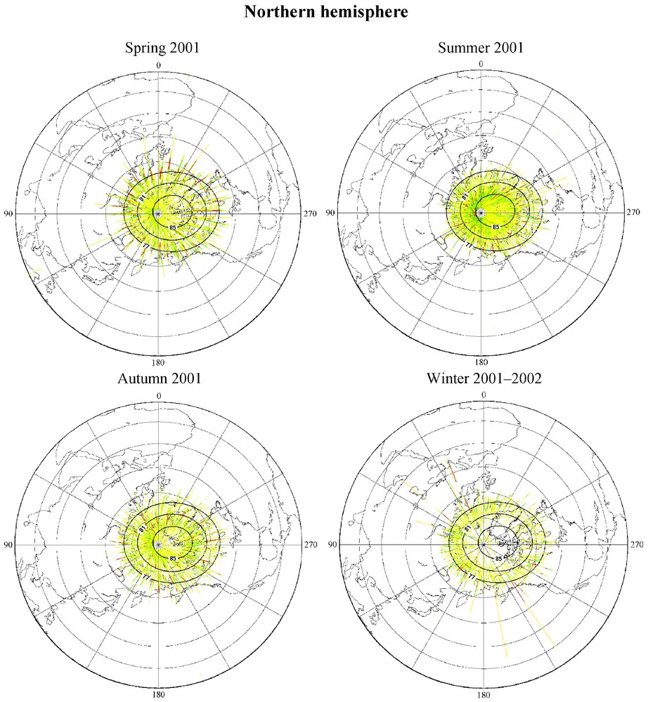
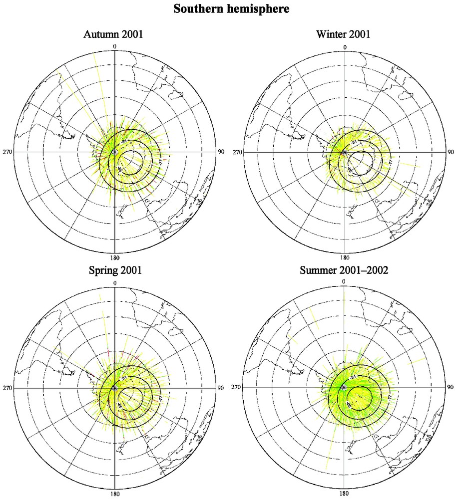
Orbit segments on which big perturbations b_t were observed: red, b_t>750 nT; green, 750>b_t>500; yellow, 500>b_t>250. Projection: polar Lambert azimutal. See main text for a remark about density of coloured segments.
Segments d'orbite sur lesquels de grandes perturbations b_t ont été observées: rouge, b_t>750 nT; vert, 750>b_t>500; jaune, 500>b_t>250. Projection polaire Lambert azimutale. Voir le texte principal pour une remarque quant à la densité des segments colorés.

5 Discussion

La figure montre les résultats obtenus pour quatre séries de 91 jours centrés respectivement sur le 21 mars 2001, le 21 juin 2001, le 21 septembre 2001 et le 21 décembre 2001. Un premier résultat spectaculaire apparaı̂t : une variation saisonnière de la distribution des perturbations, de marche opposée dans les deux hémisphères. Un second résultat est que la région colorée en jaune est localisée, pour sa plus grande partie, à l'intérieur de l'isocline 81° du système de coordonnées géomagnétiques corrigées (CGM). Le phénomène illustré par la Fig. 1 diffère radicalement de la variation saisonnière de l'activité magnétique dont l'origine se trouve sur la zone aurorale et qui est plus grande le soir. Il ne peut être relié qu'à l'activité magnétique de jour de l'intérieur des zones aurorales décrite par l'un de nous [6]. Le phénomène était alors interprété comme dû à la pénétration du vent solaire dans les « cornes » introduites par Chapman et Ferraro dans leur théorie des orages magnétiques. Les perturbations mesurées à l'altitude du satellite sont-elles bien engendrées par des courants alignés résultant de la pénétration du vent solaire ? Nos observations, nous semble-t-il, ouvrent la voie à des recherches nouvelles sur l'existence de courants alignés dans les « cusps » de la magnétosphère.

1 Introduction

It has been known for more than two decades that magnetic field measurements made aboard low altitude satellites evidence big perturbations in high latitude regions, superimposed on the smoother main field of internal origin; their amplitude reaches several hundreds of nT (see, e.g., [3,10] for recent studies relying on Ørsted satellite data). These perturbations are attributed to the so-called field-aligned currents (FAC). When computing models of the main field, the measurements from high latitudes (L>50°) are simply ignored, except for the intensity ones (e.g., [8]); the magnetic fields generated by field-aligned currents are indeed supposed to be perpendicular to the main field and consequently not to affect seriously its intensity (but see Section 4). A lot of work has of course been devoted to field-aligned currents and their magnetic effects (e.g., [2]). But it seems that researchers have focussed on individual storms or particular sources of FAC rather than on global or statistical studies.

In this paper, using a very simple technique, we will study from satellite data the global distribution of large magnetic perturbations in high latitudes, in both hemispheres. The geographical distribution of the perturbations, together with the seasonal variation of this distribution, raises some important questions about their origin.

2 The CHAMP satellite

The German satellite CHAMP was launched on 15 July 2000 into an almost circular near polar orbit (inclination 87.3°), with an initial altitude of about 450 km [8]. During the period of the present study, the satellite had an orbit repeat cycle of approximately 3 days (or, equivalently, the longitude change between two successive nodes is approximately 7°). The satellite is equipped with an Overhauser proton magnetometer and a tri-axial fluxgate sensor. For our present purpose, it is enough to say that the accuracy of the measurements is better than 1 nT.

3 The main-field model

In order to study the magnetic fields of external origin, we subtract from the measurements (see Section 4) a model of the internal, or main field. We use a Ørsted model [5], i.e. a model based on the data of Ørsted satellite, launched in February 1999 and still in operation (no model based on CHAMP data has yet been published; we could have computed one, but an Ørsted model goes as well). The main field is represented as the gradient of a spherical harmonics expansion of degree 14 (224 terms). The expansion is relative to 1 January 2000; it can be extrapolated to the time of CHAMP measurements using a secular variation term computed by Langlais et al. [5] from observatories data. We will denote the main field of internal origin ${\vec{B}}_{p} (\vec{r}, t), \vec{r}$ being the current point and t the time. The Langlais et al.'s model also contains an external field, in fact a uniform field, representing the mean effect of the ring current. This uniform external field is the only one that can safely be derived from the data; its order of magnitude is 20 nT. Let $\vec{D} (\vec{r})$ be this field; we will subtract ${\vec{B}}_{m} (\vec{r}, t) = {\vec{B}}_{p} (\vec{r}, t) + \vec{D} (t)$ from the measured field. The model field ${\vec{B}}_{m}$ represents the sum of the main field and of the average ring current field with an accuracy of 10 nT, according to the authors (Mandea, personal communication). This estimate is not critical here.

In the present study, we use the database provided by the GeoForschungsZentrum (GFZ). It contains the values of X (North component), Y (East component) and Z (vertical component) measured every second (∼10 km along orbit) by the vectorial magnetometer, and of $B = | \vec{B} |$ measured by the Overhauser sensor, as well as the time t of measurement and the corresponding longitude, spherical co-latitude and distance to the centre of the Earth.

4 The analysis

We just take the data from the file, continuously along time and trajectory:

ϕ (t), θ (t), r (t), X_{0} (t), Y_{0} (t), Z_{0} (t)

t being reckoned in seconds (subscript ‘0’ stands for observed) and, at each time moment t, we compute the differences:

Δ X (r, θ, ϕ, t) = X_{0} (r, θ, ϕ, t) - X_{m} (r, θ, ϕ, t)

(1)

for the north component, and the same for ΔY and ΔZ.

As we expect to observe magnetic perturbations generated by field-aligned currents (FAC), we compute:

(a) the intensity of the perturbation $\vec{b} (Δ X, Δ Y, Δ Z)$ ,
$b = | \vec{b} | = {(Δ X^{2} + Δ X^{2} + Δ Z^{2})}^{1 / 2}$
(b) the intensity of the longitudinal (along field) component of the perturbation,
$b_{l} = |\vec{b} . \frac{{\vec{B}}_{m}}{B_{m}}| (b_{l} \approx B_{0} - B_{m})$
(c) the intensity of the transversal component of the perturbation,
$b_{t} = |\frac{{\vec{B}}_{m}}{B_{m}} \land \vec{b}|$ (2)

In the present note, we will focus on the b_t component, the largest one (but b_l is not small either).

We represent the transverse component b_t in the following way. If b_t(t)>750 nT, the corresponding point P in Fig. 1, of coordinates (ϕ(t),θ(t)) is printed in red; if 750>b_t(t)>500, the point P(t) is printed in green; if 500>b_t(t)>250, it is printed in yellow (note that we do not discriminate altitudes). The maps and their captions make this simple procedure easily understandable.

Remark

Even for a uniform distribution of measurement points along the track, the density of these points when projected on the stereographic representations of Fig. 1 is not uniforme the density is higher, close to the geographic poles (we recall that CHAMP inclination is 87.3°). This is not a serious drawback here, where we essentially compare the geographical distribution of b_t at different epochs, in the same projection.

5 Discussion

Fig. 1 displays the obtained results for four series of 91 days, centred respectively on 21 March, 21 June, 21 September 2001 and 21 December 2001; the season names reported on the diagrams are the ones used in the corresponding hemisphere (summer in the southern hemisphere is centred on 21 December).

A spectacular result first shows up, i.e. a seasonal variation, opposite in the two hemispheres. Second, the regions coloured in yellow are essentially located inside the 81° isocline in corrected geomagnetic coordinates (CGMs; [9]) at the satellite altitude (CGMs are calculated at the date of observations); contours of the isoclines, which are different in each hemisphere and differently located with respect to the geographical poles, delineate nicely the phenomenon extension. These observations by themselves give confidence in the physical significance of the computed perturbations. The phenomenon illustrated by the maps in Fig. 1 differs radically from the semi annual variation of magnetic activity whose origin is on the auroral region and is larger in the evening. It can only be related to the midday magnetic activity inside the auroral regions, as described by one of us [6] (cf. note): it was then interpreted as due to the solar wind penetrating the horns introduced by Chapman and Ferraro in their theory of magnetic storms (now denoted magnetic cusps). The question to be answered is whether the observed perturbations at the satellite altitude are generated by field-aligned currents resulting from the solar wind entering the cusps.

Nevertheless, some of the FAC effects should rather be attributed to a proper auroral activity, in particular the one observed, in the winter of each hemisphere, between isoclines 77° and 81°. Such should also be the case for the signal observed in the same ring at the other seasons since no annual variation similar to the one observed inside the auroral zone appears.

Another observation is that the signal is globally stronger in the Northern hemisphere than in the Southern one. A first reason for this dissymmetry is that the Northern region of interest is closer to the geographic pole than the Southern one; an artefact results, due to the lesser density of satellite tracks in the Southern region. But it is also possible that a genuine physical effect contributes to the dissymmetry, due to the larger intensity of the magnetic field in the Southern hemisphere [1].

In any case, the observations that we present here seem to introduce a significant research on the existence of FAC in the cusps of the magnetosphere. Furthermore, it would be interesting to search, by a radar technique, whether a correlation exists between the ionospheric variations along the vertical of observatories located inside the auroral zone and the magnetic field perturbations with time constants of a few minutes observed at ground level on daytime.

Note

Let us recall that, when trying to interpret the 1951 recordings of the Port-Martin Antarctic station, Mayaud had to use other observations – i.e. the observations of the two international polar years 1882–1883 and 1932–1933, and the ones from a few permanent observatories such as Godhavn and Thule. In the process of describing the spatial distribution of the midday activity, he realized that the magnetic dipole coordinates were quite improper. So, using the only data available at this time, Vestine's ones, he built a coordinates system based on field values taken at the altitude of 5000 km; later on, as soon as he got aware of Hultvisq's work [4], he replaced it by what was a first sketch of the present corrected geomagnetic coordinates [7]. Note that the yellow area in maps of Fig. 1 goes beyond the 81° isocline, which he estimated as the limit of the midday activity phenomenon.

Acknowledgements

We thank the GFZ CHAMP team for providing us with the data and Mihail Roharik for discussions and help in the drawings.