

1 Introduction
The Earth's magnetic field is used as a basis for probing the Earth's lithosphere and deep interior and understanding solar-terrestrial coupling; it is also a tool for navigation, directional drilling, mineral exploration, geomagnetically induced currents and satellite operations. The geomagnetic field is mainly generated by a geodynamical mechanism in the liquid, metallic, outer core. To this dominant part of the Earth's magnetic field must be added the lithospheric contribution due to rocks that formed from the molten state and thus contain information about the magnetic field at the time of their solidification. In addition, a third important contribution is produced by the solar wind varying in intensity and speed with the amount of Sun surface activity encountering the Earth's magnetic field, known as external field.
Measurement of the geomagnetic field at a given time and location combines the resulting value of fields having different origins, as discussed above, namely: (1) the core field known also as the main field, generated in the fluid outer core, (2) the lithospheric field, generated by magnetized crustal rocks, (3) the external field, generated by ionospheric and magnetospheric currents, and (4) the electromagnetic induction field, generated by currents induced in the crust and the mantle by the time-varying external field. Separating these contributions is not an easy task [20]. However, in 1838, C.F. Gauss, using spherical harmonic expansion of the geomagnetic field, developed a method to describe the geomagnetic field globally, providing a rough separation between internal and external contributions to the field.
The geomagnetic field is also subject to temporal variations over various time scales. The so-called short-term variations are detectable over time scales ranging from ∼0.01 s to decades. The very short period variations (seconds to hours) are usually attributed to the Earth's external sources, while the longer-period variations (annual to decadal) are due to solar cycle variations and its harmonics, superposed on the core field temporal variation. The latter is known as the secular variation.
Observations of the full vector magnetic field exist for more than a century, with the first magnetic observatory installed by C.F. Gauss in Göttingen, in 1832. In addition to the observatory network, vector measurements provided by satellites and available since 1979 have greatly improved our knowledge of the geomagnetic field all over the globe. In the following sections, a discussion about the different kinds of measurements is provided, with an emphasis on the role of the latest satellite missions, Ørsted, CHAMP and SAC-C, for providing a better description the Earth's magnetic field.
2 Measuring the Earth's magnetic field: from ground-based observatories to satellite missions
Historically, the role of magnetic observatories was to monitor the secular change of the geomagnetic field, and this remains one of their most important tasks. Some observatories installed at the end of 19th century, provide, nowadays, long-time series. An example is the Chambon-la-Forêt observatory series, covering a total time span of 123 years when the present site measurements (1936–present) are combined with prior nearby measurements made in Saint-Maur (1883–1900) and Val-Joyeux (1901–1935). Today, some 200 observatories are operated worldwide (Fig. 1). To run a magnetic observatory generally involves continuous variation measurements of three field components (one-minute or even one-second data sampling), which are recorded automatically by fluxgate magnetometers. However, these instruments are subject to drifts arising from sources both within the instrument (e.g., temperature effects) and the stability of the instrument mounting. These measurements do not provide absolute values and the instruments are known as variometers. Absolute measurements of the full vector field, sufficient in number to control the instrumental drift, are necessary to calibrate the variometer recordings. Modern land-based magnetic observatories all use similar instrumentation to produce similar data products. For a full description, see [12] and also the INTERMAGNET web site (http://www.intermagnet.org). The fundamental measurements recorded are one-minute values of the vector components and scalar intensity. The one-minute data are important for studying variations in the external magnetic field, in particular the daily variation and magnetic storms. From the one-minute data, hourly, daily, monthly and annual mean values are produced. The monthly and annual mean values are used to determine the secular variation originating inside the Earth's core. The quality of secular-variation estimates therefore critically depends upon the quality of the absolute measurements at each observatory.
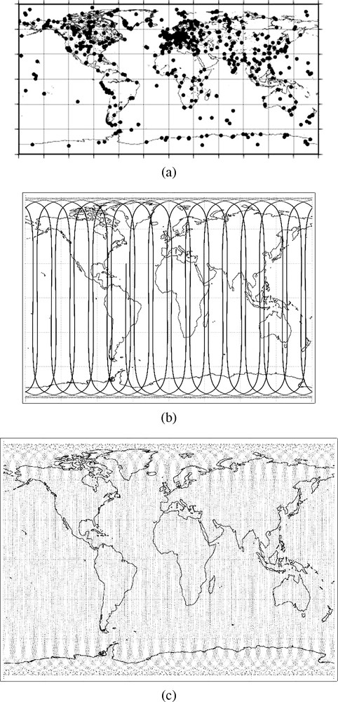
Global distribution of magnetic data provided by (a) all 671 observatories ever run, even if they provided only a single annual value, (b) CHAMP satellite tracks over one day, (c) CHAMP satellite tracks over one week. For the magnetic observatories, the distribution is seen to be highly non-uniform, with the Northern hemisphere better covered than with the Southern hemisphere. For the satellite, the coverage over one week appears already sufficient for an adequate data distribution; note that these plots are based on all available measurements, without considering data quality and selection criteria.
Distribution globale des données géomagnétiques. (a) L'ensemble des 671 observatoires qui ont fonctionné, y compris s'ils n'ont fourni qu'une valeur moyenne annuelle. (b) Traces au sol des orbites CHAMP pendant une journée. (c) Traces au sol des orbites CHAMP pendant une semaine. Dans le cas des observatoires, il est aisé de remarquer la non-uniformité des distributions, l'hémisphère nord étant mieux couvert que l'hémisphère sud. La couverture satellitaire d'une semaine paraît suffisante pour obtenir une distribution de mesures exploitable. Cette distribution ne tient cependant pas compte de la qualité des données et des critères de sélection.
Since the 1960s, the Earth's magnetic field intensity has been measured intermittently by satellites. Only recently have there been several missions dedicated to measuring the full field vector, using star cameras to establish the direction of a tri-axial fluxgate sensor. An absolute intensity instrument is also carried to calibrate the vector instrument, and both magnetic instruments are kept remote from the spacecraft by mounting them at the end of a few metre-long non-magnetic boom. The first satellite that provided valuable vector data for geomagnetic field modelling was the MAGSAT mission [14], which resulted in magnetic measurements over a six-month period, between 1979 and 1980. The following 20 years were without satellite magnetic coverage. However, in recent years, the geomagnetic community has been provided with a wealth of new high-quality data from several near-Earth satellites, Ørsted (1999–present), CHAMP (2000–present) and SAC-C (2000–present).
The Danish Ørsted magnetic satellite launched in 1999 is still operational. The satellite carries as its primary scientific payload a tri-axial fluxgate magnetometer and a star camera for measurements of the geomagnetic field. Its position is acquired using Global Positioning System (GPS) receivers. The orbit is inclined 98° to the Earth's equator, resulting in a precession of the orbital plane relative to the direction to the Sun. This precession allows the mapping of almost the entire globe as the Earth rotates. The spacecraft main body carries the electronics while an 8-m boom hosts the magnetic-field instruments. The Ørsted satellite takes about 100 min to orbit the Earth in its near-polar orbit. The local time of the orbit changes by 0.9 min day−1, and the data are from an altitude range of 640 to 850 km. The Ørsted Overhauser magnetometer measures the scalar values of the magnetic field with an accuracy of <1 nT, while the fluxgate magnetometer together with the star camera provides vector data with a precision of <3–5 nT [24].
CHAMP (Challenging Minisatellite Payload) was launched in July 2000. With its highly precise, multifunctional and complementary payload elements (magnetometer, accelerometer, star sensor, GPS receiver, laser retro reflector, ion-drift meter) and its orbital characteristics (near polar, low altitude, long duration), CHAMP currently provides high-precision gravity and magnetic-field measurements. The spacecraft has a length of 8.33 m (including the boom). With an orbital period of 93 min, and an initial altitude of 454 km, the satellite moves rapidly through local time, with a change of 5.45 min day−1. Both magnetic fluxgate sensors are mounted together with the star cameras on a common optical bench providing a mechanical stability between these systems of better than 20 arcsec. The optical bench is located about 2 m away from the spacecraft main body, while the Overhauser magnetometer is at the end of the 4-m boom. This configuration results from a compromise between avoidance of magnetic interference from the spacecraft and cross-talk between the vector and scalar magnetometers. The almost circular and near-polar orbit (87.3° with respect to the equator) allows a homogeneous and almost complete global coverage of the Earth, as required for gravity and magnetic measurements. The CHAMP scalar magnetometer provides an absolute in-flight calibration capability for the vector magnetic-field measurements. A dedicated program ensuring the magnetic cleanliness of the spacecraft allows an absolute accuracy of <0.5 nT for the intensity data. The scalar calibration using the absolute Overhauser observations is run on a daily basis and the input parameter set for the fluxgate processing is updated every two weeks. The corrections applied to the data are based on sensor sensitivities, misalignments, offsets, static-time adjustments, and satellite fields [24,25].
SAC-C (Satelite Argentino de Observacion de la Tierra) was launched in the same year as CHAMP, and is a joint Argentinian–US mission that hosts a Danish–US magnetometry package. SAC-C has a circular orbit at 702-km altitude, an inclination of 98.2° and the Sun-synchronous orbit crosses the equator at 10:24 and 22:24 Local Times. The same package as for Ørsted is mounted on the SAC-C spacecraft, but the vector data cannot be used, as the star camera has given no information during the course of the mission, possibly because of a cabling problem on the boom. As a consequence, magnetic-field measurements from SAC-C are restricted to the 1 Hz values from the scalar Helium magnetometer, with an accuracy of better than 4 nT. This higher value is partially due to the uncertainty of the spacecraft fields.
3 Magnetic data
3.1 Spatial data distribution
The distribution of magnetic observatories about the globe is highly non-uniform with the Northern hemisphere having better coverage than the Southern hemisphere (Fig. 1a). The observatory distribution is a key parameter in determining the secular variation on a global scale. This is the reason why, in some regions, for example, the Pacific Ocean, the secular variation uncertainty is in the order of hundreds of nT yr−1 [19], while in better-covered regions such as Europe, it is a few nT yr−1. An alternative for improving our knowledge of the secular variation is to have well-distributed global measurements provided by satellites. The data provided by each of the three satellites currently in orbit ensure good coverage of the Earth's surface in a very short period of time. Fig. 1, for example, shows also the CHAMP satellite tracks coverage after one day (Fig. 1b) and one week (Fig. 1c), respectively. The coverage after one week already appears sufficient for a good data distribution. However, these plots are based on all available measurements, without considering data quality and selection criteria, which are important for geomagnetic field modelling.
3.2 Temporal coverage
Since the first magnetic observatory installation, their number has continuously increased. However, the number of observatories providing annual means is different from those providing hourly means or one-minute data. The temporal distribution of these three kinds of datasets provided by the magnetic observatories varies in time, and a few milestone epochs are indicated in Table 1.
Number of observatories which provide: a annual and b hourly means, and c one-minute values for a few milestone epochs (at 1 January 2005)
Nombre d'observatoires qui fournissent des moyennes a annuelles et b horaires, et c des valeurs sur une minute pour des époques étapes (au 1er janvier 2005)
| Epoch | AMa | HMb | 1-minc | Remarks |
| 1833 | 1 | 0 | 0 | Gauss installed the first magnetic observatory |
| 1883 | 39 | 0 | 0 | The French observatory was installed |
| 1900 | 55 | 1 | 0 | Beginning of the 20th century |
| 1933 | 100 | 26 | 0 | The first time 100 observatories are in operation |
| 1958 | 170 | 114 | 0 | The International Geophysical Year, IGY |
| 1987 | 192 | 112 | 36 | The maximum of annual means are available |
| 2000 | 163 | 131 | 105 | Beginning of the 21st century |
The time span covered by the satellite missions is, in comparison, very short. Table 2 summarizes the magnetic satellite missions mainly used for studying the Earth's internal and external fields. However, if we consider only satellites providing high-accuracy vector data in a near-Earth orbit, the number of satellite missions is reduced to only four.
Magnetic satellite missions: a inclination in degrees; b altitude in km; c accuracy in nT
Missions satellitaires d'observation magnétique : a inclinaison en degrés ; b altitude en km ; c précision en nT
| Name | Period | Inc.a | Alt.b | Acc.c | Remarks |
| Cosmos 49 | 1964 | 50 | 261–488 | 22 | Scalar |
| OGO-2 | 1965–1967 | 87 | 413–1510 | 6 | Scalar |
| OGO-4 | 1967–1969 | 86 | 412–908 | 6 | Scalar |
| OGO-6 | 1969–1971 | 82 | 397–1098 | 6 | Scalar |
| MAGSAT | 1979–1980 | 97 | 325–550 | 6 | Vector |
| DE-1 | 1981–1991 | 90 | 568–23290 | ? | Vector (spinning) |
| DE-2 | 1981–1983 | 90 | 309–1012 | ? | Low accuracy vector |
| POGS | 1990–1993 | 90 | 639–769 | ? | Low accuracy vector |
| UARS | 1991–1994 | 57 | 560 | ? | Vector (spinning) |
| Ørsted | 1999–present | 98 | 640–850 | 3 | Vector |
| CHAMP | 2000–present | 87 | 300–454 | 3 | Vector |
| SAC-C | 2000–present | 98 | 702 | ? | Vector |
4 What new insights have novelties magnetic satellite data brought us?
The launch of the Danish satellite Ørsted highlighted the importance of satellite measurements. Using the Ørsted or/and CHAMP datasets, combined with magnetic ground observatory data, allows us to improve our knowledge of the geomagnetic field by offering a highly accurate separation of the sources over multi-year time intervals. In the following, only a few examples are given from the multitude of results recently obtained, from core to space.
4.1 Core field and secular variation
4.1.1 IGRF models
The reference global geomagnetic field model is the International Geomagnetic Reference Field (IGRF) [18]. It has been produced on a five-year timescale, the first epoch being 1900.0, from a range of measurements provided by magnetic observatories, ships, aircraft and satellites. These models, derived through a classical spherical harmonic analysis of a large amount of data, represent the magnetic field generated in the Earth's core. Even in the era of GPS navigation, the IGRF models still play a vital role, being implemented into the GPS navigation systems as a backup. The quality of this series of models has dramatically increased over the last two field generations. Indeed, with the 8th generation, the main-field models are currently defined up to spherical-harmonic degree 13, compared with a maximum degree 10 for all previous generations [19]. These models represent the first useful combination of satellite and observatory data. The satellite data, on the one hand, are needed to ensure a good distribution over the globe, while on the other, information about magnetically quiet conditions are provided by the observatories. Therefore, using both data platform types allows for developments of more reliable geomagnetic models [8,16,22].
4.1.2 Secular variation and geomagnetic jerks
Modelling the secular variation, with characteristic times the order of some years to a few decades, can be significantly expanded, owing to the two satellite vector magnetic surveys carried out by the Ørsted and CHAMP missions. These missions permit the study of the geographical pattern of the secular variation during each satellite's lifetime, and also allow a comparison with former data from the MAGSAT mission in 1979–1980 [15]. A recent model, CHAOS [26], covering more than 6.5 years, brings important improvements in describing the secular variation from satellite data. Indeed, the secular variation is no longer considered as linear, but the non-linear time changes are described by means of splines, to reduce unrealistic behaviour near the edges of the time interval. The new robust model resolves secular variation coefficients beyond degree 13, which means that it is for the first time possible to infer the temporal changes of the core field to smaller scales than the field itself and to evaluate structures with short wavelengths at the core–mantle boundary, never observed before (Fig. 2).
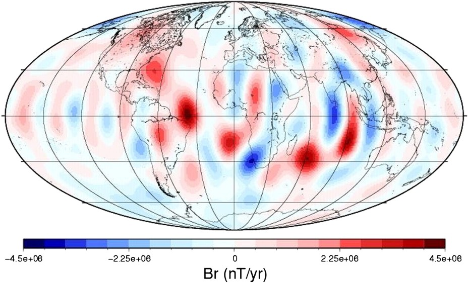
Map of the secular variation of radial field at the core–mantle boundary for epoch 2002.5. The field values are computed from a secular variation model up to degree 14 provided by [26].
Cartographie de la variation séculaire de la composante radiale du champ à l'interface noyau–manteau, pour l'époque 2002.5. Les valeurs du champ sont calculées en utilisant un modèle de variation séculaire jusqu'au degré 14 fourni par [26].
The secular variation is also characterised by a number of abrupt changes, which have been reported in magnetic observatories series. During the 20th century, some seven events have been detected and analysed [21]. The cause of these abrupt variations (spanning some months to a couple of years) are the so-called geomagnetic jerks (see for more details [1,4,17]). These features are not yet completely understood, but may reflect the contribution of hydromagnetic motions in the outer core over small scales. Recently, a possible explanation for geomagnetic jerks origin has been proposed as a combination of a steady flow and a simple time-varying, toroidal zonal flow [3], consistent with torsional oscillations in the Earth's core. Moreover, geomagnetic jerks and a high-resolution length-of-day profile have been investigated for core studies [9]. These phenomena are difficult to study, because of their small amplitudes and the overlap of their frequency range with the effect of solar-dependent external variations. In addition, the highly uneven coverage of the globe by magnetic observatories also makes their study difficult [20].
4.1.3 Southern African continent and its reversed magnetic flux
Recent studies have identified distinct patches of reversed magnetic flux at the poles and below Africa, which also account for the present-day field decrease [10]. The most prominent feature in this respect is the growing patch of reverse magnetic polarity beneath South Africa. To give an indication of the recent changes, Fig. 3 shows the distribution and evolution of the radial magnetic field component at the core–mantle boundary for four epochs during the past century. The model used here [11] shows a region of reversed field direction that propagates northeastward. A decade ago, this patch was directly below South Africa, and its directional propagation continues when recent models based on satellite data only, such as CHAOS, are used [26] (see again Fig. 3). Below the southern African continent is one of the two regions of very active variations of secular variation, where wave-like structures propagate [5,6]. The magnetic activity within these structures directly relates to the geomagnetic jerks previously reported at the Earth's surface [1,21].
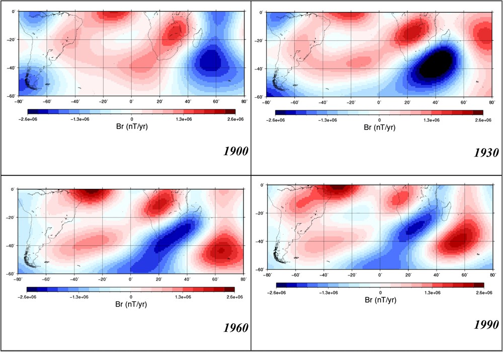
Maps of the secular variation of the radial field at the core–mantle boundary for the epochs 1900, 1930, 1975, 1990 under the South Atlantic Anomaly region. The field values are computed from a secular variation model up to degree 14 provided by [11].
Cartographie de la variation séculaire de la composante radiale du champ à l'interface noyau–manteau, pour les époques 1900, 1930, 1975 et 1990 sous de la région anomale de l'Atlantique sud. Les valeurs du champ sont calculées en utilisant un modèle de variation séculaire jusqu'au degré 14 fourni par [11].
The orientation of the geomagnetic field in southern African region is also changing rapidly. In the northwestern part of the southern African continent, the declination of the magnetic field is propagating eastward and in the southeastern part westward. This causes a spatial gradient over the subcontinent which is presently increasing with time. A greater density of observation points is required in order to resolve the structure of the field orientation and its evolution. This is one of the most significant examples supporting the need to install new observatories.
4.2 Lithospheric field
The models of the core field derived from satellite data can also be used to better describe the lithospheric contributions. Indeed, in modelling the internal contributions, both core and lithospheric fields are described by the spherical harmonic coefficients. In order to obtain the core field, degrees larger than 14 are usually discarded. To the contrary, for obtaining the lithospheric field, the degrees smaller than 14 are set to zero. A better description of the lithospheric fields and external variations is not only necessary to improve models of the core field and its secular variation, but is also of great importance for geodynamics and induction studies. However, considerable difficulties exist in carrying out a joint analysis of ground-based and satellite data, as they are characterized by different spatial and temporal distributions. Two examples presented here concern the global, and the regional modelling of the lithospheric field.
High-quality lithospheric field models from CHAMP data have become increasingly stable and reliable [23]. Unfortunately, noise hampers the modelling of the lithospheric field, and global models are not stable above degree 90, providing a 400-km maximum resolution. Recently, almost five years of CHAMP scalar and vector data (from August 2000 to January 2005) were processed using a regional modelling scheme [30]. Indeed, in order to make a better use of magnetic data from different platforms for modelling the lithospheric contributions, a new method has been recently developed and improved by [29,30]. It is based on the solution of the Laplace equation within a spherical cone, and is referred to Revised Spherical Cap Harmonic Analysis. This helps to better separate disturbed regions, such as polar regions, from quiet ones. Covering the Earth by regional patches allows the representation of the magnetic field at satellite altitudes with unprecedented accuracy. The local models are estimated using the least disturbed satellite tracks from local time sector 00:00 to 05:00. Further corrections like polar electrojet, tidal effects [13,32] and plasma bubbles [33] are also applied and a core field and a secular variation model are subtracted. Fig. 4 shows the vertical component at 400 km altitude, which displays some small features originating mainly from genuine crustal signal but not retained in a global model [30]. So far, the main drawback of the regional patchwork is the downward continuation of the local models to the Earth's surface [28].
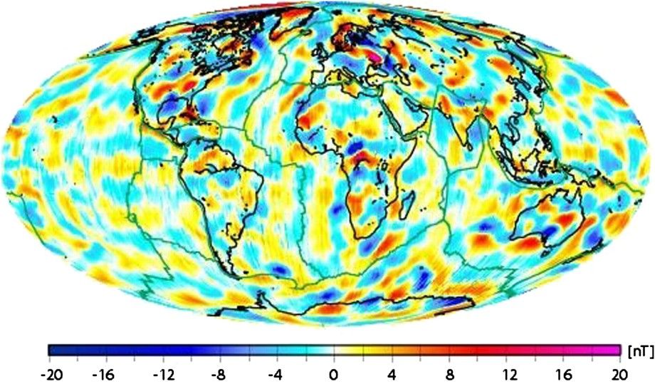
Map of the lithospheric field obtained from CHAMP satellite data when the Revised Spherical Cap Harmonic Analysis is applied [30].
Cartographie du champ lithosphérique, établie à partir des données du satellite CHAMP en utilisant l'analyse en harmoniques sur calotte sphérique de [30].
The method described above also allows the inclusion of data from different altitudes, i.e. from ground, aeromagnetic surveys and satellites, for a combined inversion. The method applied to regional modelling provides very interesting results. In the example given here the Chambon-la-Forêt observatory data, the French repeat station data, as well as the available aeromagnetic and CHAMP satellite measurements over the French Metropolitan territory are considered. Fig. 5 shows the resulting vector map for the vertical component only. The main geological structures are well defined, such as the Parisian Basin anomaly, even in this map at 40-km altitude [31].
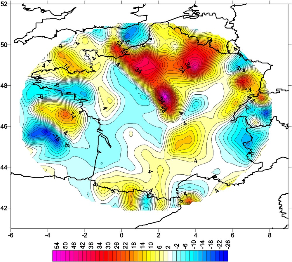
Map of the vertical component over the French territory obtained from ground, aeromagnetic and CHAMP satellite data when the Revised Spherical Cap Harmonic Analysis is applied [30]. The map is continued at 40-km altitude: the main features are still defined, as the Paris Basin anomaly (E. Thébault, pers. commun.).
Cartographie de la composante verticale du champ d'anomalie magnétique établie au-dessus du territoire français à partir des données au sol, aéromagnétiques et satellitaires CHAMP, en utilisant l'analyse régionale sur calotte sphérique [30]. Le champ est recalculé à 40 km d'altitude. Les principales anomalies, telle l'anomalie du Bassin parisien, restent encore bien définies.
4.3 External field
The development of new analysis techniques for data from satellites and observatories permits the separation of field sources, internal and external to the Earth's surface, and also into those internal and external to the region of satellite observations. Here, a single example is given with respect to the external contributions. In theory, the ionospheric sources, which are external to the Earth's surface, but internal to the satellite, can be isolated. Such a separation allows for better parameterisation of both the main geomagnetic field and the external variations which are modulated by the solar activity.
Both satellite and ground-based data are used for studying the ionospheric contribution in magnetic field measurements. The most intense current system in the ionosphere is that of the horizontally flowing auroral electrojet in the auroral oval. The strength and latitudinal position of these current flows depend on many factors, for example on the solar zenith angle, solar wind activity, magnetospheric convection and substorm processes. The characteristics of the auroral electrojet reflect the dynamics and the processes at the magnetopause and in the outer magnetosphere. The electron energy is transported from the magnetosphere to the ionosphere by currents flowing along the field lines. Their intensity controls the electric field and partially the state of ionospheric conductivity, and with it the strength and location of the auroral electrojet. Recently, the horizontal ionospheric current density from magnetic field measurements taken onboard the CHAMP satellite was computed [27] and compared with measurements taken at the ground by the IMAGE (http://www.ava.fmi.fi/image/) ground-based magnetometer network [2]. For this purpose, total field data sampled by the Overhauser Magnetometer on CHAMP and the horizontal magnetic field measurements of the IMAGE network were used. The high correlation of the current curves demonstrates the capability of ground-based observations at high latitudes to predict the strength of the electrojet signatures in the satellite magnetic field scalar data.
5 Conclusion
To map both the spatial and temporal variations of the geomagnetic field, data from surface observatories, special land and sea surveys, and from satellites have to be jointly used. During the last few years, several new satellites (Ørsted, CHAMP, SAC-C) were launched by different agencies to measure the Earth's magnetic field from near-Earth orbit; their data are made available by each of the mission data centres. For scientists, a major benefit of this high-quality and huge amount of magnetic measurements, from ground and space, is to get better insight of the hidden interior of the planet, and its place in the magnetic solar system.
Without doubt, the latest magnetic satellite data have brought by themselves new highlights on the Earth's magnetic field. The new field models bring important improvements in describing the internal magnetic sources. One of the most remarkable improvements in the knowledge of the core field is our ability to map small-scale structure of the secular variation, resolving linear secular variation up to degree 15 [26]. The lithospheric field exceeds the core part for spherical harmonic degrees above 13, and it is therefore not possible to infer small-scale structure of the core field. The three magnetic missions, Ørsted, CHAMP and SAC, allow for the first time inference of the secular variation of the core field down to smaller scales than the (static) core field itself. Another major improvement relates to the lithospheric field. The high-quality satellite data lead to a detailed representation of the lithospheric field, up to degree 90 [23]. The difference between MAGSAT and CHAMP epochs, and corresponding models is due to significantly improved data accuracy and to the longer observational period [20].
The geomagnetic field is shielding our habitat from the direct influence of solar activity which becomes apparent during strong geomagnetic storms when the shield is pushed earthward under the influence of the high-speed solar wind. These magnetic storms often lead to satellite failures, problems in telecommunication and radio transmission or even regional power failures are often encountered as consequences of them. To map the geomagnetic field with both its spatial and temporal variations, and on different scales, is essential to understand it, and to better forecast what will be the space weather of tomorrow!
Our magnetic planet will remain under observation with the European Space Agency's forthcoming Swarm mission. Three satellites will be launched in 2010 and will measure the magnetic field and its variations far more accurately than ever before [7]. However, a comprehensive separation and understanding of the internal and external processes contributing to the Earth's magnetic fields is possible only by joint analysis of satellite and ground-based data, with all the difficulties combining such different datasets entail. Continuous space-borne and ground-based monitoring of the magnetic field aims to address this need.
Acknowledgements
All figures were produced with GMT [34]. I would like to thank Anny Cazenave for inviting me to contribute with the present work. I would also like to thank Richard Holme, Aude Chambodut, Mohamed Hamoudi, Patricia Ritter, Martin Rother, Erwan Thébault for discussions and help with graphics.