

1 Introduction: The dilemmas of deep uncertainty
An advisory group charged with the role of summarising scientific knowledge for policy purposes, the Intergovernmental Panel on Climate change (IPCC) faces a difficult challenge. As a scientific body the IPCC needs to be true to the objective norms of science and scientific practice. Since credibility of IPCC assessments within the scientific community is a necessary condition for its success, IPCC reports have to assess as accurately as possible the current state of scientific knowledge as evidenced in the literature. In its role as a policy advisory committee, however, the IPCC goes beyond the routine bounds of scientific convention and provide a synthesis of the state of the science in order to inform the UN Framework Convention on Climate Change. The inter-governmental policy-making community, who is the client of the IPCC reports, wants answers to questions that objective science alone cannot answer. Yet, the relevance of the IPCC hinges on the provision of such policy relevant information.
To date, the IPCC has been reasonably successful in navigating this tension between credibility of its science and relevance of its assessment. It has done so by instituting an assessment framework that is ‘co-produced’ by scientists, bureaucrats and policy makers [21,22]. It has also instituted a rigorous and transparent review process that involves both scientists and members of the policy community [6]. One area where the IPCC has been less successful in meeting the demand for policy relevant information is in the assessment and communication of uncertainties [19]. Some of this lack of success is due to the very nature of the issue. There is deep uncertainty1 in the climate problem that originates from the long time scales and complexity. Further, there has historically been little debate within IPCC's diverse inter-disciplinary scientific community on whether and how best to reason about and communicate uncertainties.
There are two markedly different approaches to uncertain reasoning. Those in the frequentist camp assign probabilities based strictly on observational counts. So, in responding to the question “what is the chance that it will rain tomorrow?”, frequentists restrict themselves to historical data. A Bayesian on the other hand is likely to modify climatological predictions with expert judgement, model predictions or other subjective data in providing an answer to the same question. Likewise, IPCC statements that the global average surface temperature has increased, over the 20th century, between 0.4–0.8 °C, with a 95% confidence are closer to the frequentist paradigm, while those that venture to predict future outcomes of the same quantity use some form of Bayesian reasoning.2
Formal consideration of uncertainty in the IPCC assessments that began with the Third Assessment Report (TAR) largely followed a Bayesian paradigm.3 As a part of the TAR process, Moss and Schneider [16] wrote a guidance document that developed a common schema for representing and communicating uncertainty in both quantitative and qualitative terms across all three working groups. The use of the schema in the TAR was mixed with some working groups (notably WG-1) using it more often than others. There were also criticism of the TAR for not “adequately treating uncertainty in those conclusions that are most important for policy decision-making” [19]. Criticisms notwithstanding, the Moss and Schneider proposal was successful in raising the profile of uncertainty in the IPCC process.
As the IPCC works to improve the representation of uncertainty in the Fourth Assessment Report (AR4), several issues on the role and nature of uncertainty will need to be addressed. Some of these are operational and more or less limited to narrow issues of representation in IPCC documents: what is the best way to define risk and uncertainty? Should all working groups have a similar/common approach to communication of uncertainties? Should linguistic scales be used? If so, how many levels of scales are best? These and other similar questions have begun to be discussed in the emerging literature [5,15].
There is, as we describe below a more fundamental issue – a camel in the uncertainty tent – that has received less attention. In order to generate policy-relevant knowledge, the scientific community is willingly or otherwise engaged in subjective analyses. Projections and predictions used for policy analysis incorporate subjective knowledge making strictly frequentist approaches difficult to sustain. Bayesian approaches have become par for the course in the assessment of risks in other areas of risk research and climate is unlikely to be an exception. However, two persistent criticisms of the Bayesian approach going back to its earliest days remain [24] and are all the more salient in climate-change assessment because of the presence of deep uncertainty. The difficulty of coping with deep uncertainty in a Bayesian framework manifests itself through two problematic assumptions:
- • precision: the doctrine that uncertainty may be represented by a single probability or an unambiguously specified distribution;
- • prior knowledge of sample space: the assumption that all possible outcomes (the sample space) and alternatives are known beforehand.
These issues raise questions that are epistemological in nature and go to the heart of the scientific approach: how can scientists articulate, analyze and communicate uncertainties in the face of deep uncertainty and ignorance, i.e., when there is a profound lack of understanding and/or predictability? How can knowledge about scientific consensus or disagreements be communicated in a manner that reflects the actual degree of consensus within the community? How might one analyze and communicate uncertainty about uncertainty, i.e., what should be done when probabilities are imprecise?
This paper reflects on the latter set of questions. In particular, we focus on how different levels of knowledge can be meaningfully represented so as to reflect the range of incertitude from ignorance to partial ignorance to uncertain knowledge. We argue that existing schemes do an inadequate job of communicating about deep uncertainty and propose a simple approach that distinguishes between various levels of subjective understanding in a systematic manner.
One way in which deep uncertainty can be formalized is by using concepts of probability imprecision and ignorance. Thus, lessons for communicating uncertainty in the face of probability imprecision and ignorance are also likely to be useful for communicating deep uncertainty. Thus in Section 2 we examine the literature on decision making for insights coping with ignorance and probability imprecision (ambiguity). In Section 3, we present examples from the climate change literature that attempt, in our view unsuccessfully, to communicate issues of deep uncertainty and ignorance. In Section 4 we develop and demonstrate a methodology for representing deep uncertainties. We end with a discussion of the implications for the IPCC.
2 Imprecise probability: ambiguity and ignorance
Formal decision-making frameworks require the explication of three quantities – an outcome variable, probability of that outcome variable, and utility of the outcome variable.4 In typical decision models these quantities are precisely known. The decision theoretic literature provides several analytical ways of coping with imprecise probability (or ambiguity) that in its most extreme form results in ignorance, i.e., the inability to provide probability measures on regions of the sample space5 [3]. While these mathematical techniques provide the tools to address imprecision in prescriptive models, they tell us little about how imprecise probability can be best communicated in practice. There is more success to be gained from descriptive approaches taken from the literature on psychology of decision-making.
Empirical studies of how people deal with probability imprecision have tended to focus on situations where probabilities are imprecise, but outcomes and utilities are known [13]. There are also some studies that deal with imprecise utilities and partly known outcomes [9], and very few studies that address sample space ignorance. Though limited these studies provide a few insights into human responses to imprecise probability, and help us in developing plausible strategies for communicating imprecise probability and outcome information. These insights are outlined below.
2.1 Ambiguity aversion
Ambiguity aversion refers to the observation that people prefer an outcome whose probability is precisely specified to an outcome associated with imprecise probability even when the two outcomes are identical in a rational sense. There is also strong evidence that ambiguity aversion is distinct from risk aversion [3]. In other words, people tend to value reduction in ambiguity for its own sake.
2.2 Conflict aversion
Smithson and colleagues have performed studies that provide strong support for the hypothesis that people prefer consensual but ambiguous assessments to disagreeing but precise ones, and that they regard agreeing but ambiguous sources as more credible to disagreeing but precise ones [23]. Thus, communicating the manner in which expert views are incorporated into the IPCC may be as important as actual choices of tools for uncertainty communication.
2.3 Ignorance aversion
Experimental psychology provides relatively few insights into how humans cope with sample space ignorance in decision-making. Fischhoff et al. [7] showed that people tend to underestimate probabilities of ‘catch-all’ categories for outcomes. Tversky and Koehler [25] have shown that unpacking a compound event into disjoint components tends to increase the perceived likelihood of that event. Thus, in contradiction with the basic axioms of probability, more ‘refined’ knowledge of an event might lead to greater perceived probability of its outcome. While specific insights from the study of ignorance aversion to the issue of uncertainty communication are sparse, this literature presents one broad insight – when communicating ignorance the level of detail (even not very relevant detail) in information provided is important [24].
These three phenomena can be used to provide some preliminary guidelines for how deep uncertainty might be communicated. Ambiguity aversion suggests that care needs to be taken when providing information about imprecise probabilities. People are more likely to make choices that depart from the rational when confronted with imprecise probabilities. Thus, if deep uncertainty can be conveyed without explicitly invoking imprecise probability, then people might be better able to rationally interpret that information. The presence of conflict aversion suggests that careful attention needs to be paid to the generative causes of ambiguity, with implications for how ‘traceable accounts’ [16] for uncertainty assessments are produced. If ‘traceable accounts’ are produced from a consensus-based process, they are more likely to be trusted even if they convey less precision. Finally, ignorance aversion suggests that simple schemes that attempt to represent uncertainty in a uniform manner across many different contexts (such as the Moss and Schneider scale) may lead to biases when depending on how much detail is presented in the information.
3 The difficulties of communicating probability imprecision: two examples from the climate change literature
The literature on representation of uncertainties in climate change does not explicitly recognize the issue of probability imprecision. However, there are examples in the literature demonstrating how scientists are coping with deep uncertainties of climate change by invoking imprecision. In what follows we present two such examples and argue why they may be inadequate tools for communication.
3.1 Example 1
The IPCC TAR working group 1 report [12] presents a novel way of representing uncertainty in radiative forcing from several sources. The diagram (shown in Fig. 1) appears in both the technical summary of the scientific assessment and in the relevant chapter (Chapter 6).
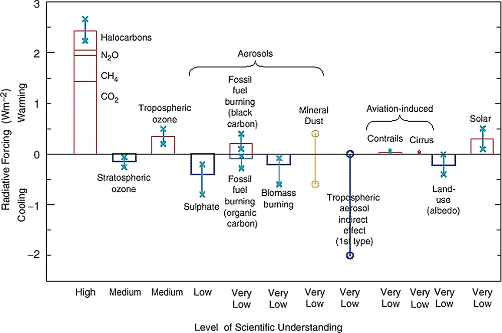
This figure is taken from the IPCC TAR. Global, annual-mean radiative forcings (W m−2) due to a number of agents for the period from pre-industrial (1750) to present (late 1990s; about 2000) The height of the rectangular bar denotes a central or best estimate value, while its absence denotes no best estimate is possible. The vertical line about the rectangular bar with × delimiters indicates an estimate of the uncertainty range, for the most part guided by the spread in the published values of the forcing. A vertical line without a rectangular bar and with ○ delimiters denotes a forcing for which no central estimate can be given, owing to large uncertainties.
Cette figure est empruntée au troisième rapport d'évaluation du GIEC. Forçages radiatifs moyennés sur un an et sur l'ensemble du globe, découlant d'un certain nombre de facteurs depuis la période préindustrielle (1750) jusqu'à l'époque actuelle (fin des années 90, environ 2000). La hauteur des rectangles indique la valeur centrale ou la meilleure estimation, l'absence de rectangle indiquant l'impossibilité de proposer une meilleure estimation. La barre verticale sur un rectangle, délimitée par des ×, indique une estimation de la marge d'incertitude, faite essentiellement sur la base de la dispersion des forçages publiés. Une barre verticale sans rectangle et limitée par des ○ dénote un forçage, dont la valeur moyenne ne peut être indiquée en raison d'incertitudes trop importantes.
Notice that the figure includes a “level of scientific understanding” (LOSU) index for each forcing (high, medium, low and very low). These are subjective judgments “about the reliability forcing estimate, involving factors such as the assumptions necessary to evaluate the forcing, the degree of knowledge of the physical/chemical mechanisms determining the forcing, and the uncertainties surrounding the quantitative estimate of the forcing” [1]. Where the same figure appears elsewhere in the report we are also told that “the uncertainty range specified here has no statistical basis and therefore differs from terms used elsewhere in the document” [18].
This figure encapsulates several of the dilemmas that scientists face in communicating deep uncertainty in IPCC reports. Clearly the authors were uncomfortable with providing statistical meaning to the uncertainty bounds presented in Fig. 1, hence the disclaimer that the range specified has no statistical basis. The LOSU scale provides a second layer of hedging against interpretation of the uncertainty ranges by conveying an added level of imprecision. From the perspective of a policy analysis such communication is not very useful. First, there is no guidance on how to interpret the uncertainty range. Indeed no statistical interpretation of the range is provided. Further, even if an analyst were bold enough to use his own subjective judgment and ascribe a probabilistic interpretation to a forcing agents range, the “very low” LOSU scale for 75% of the agents makes it hard to make a consistent interpretation. More generally, with the exception of forcing agents with high LOSU levels, such representations of uncertainty are very difficult to interpret. This form of representing uncertainty introduces imprecision at multiple levels – first, by not providing a probability based interpretation of radiative forcing of agents ambiguity is created; and second by providing the LOSU scale as a hedge further incertitude is introduced. Some of this imprecision is unavoidable, especially when scientific information needed to make more definitive statements does not exist. Yet as we demonstrate in Section 4 it is possible to cope with deep uncertainty in a way that makes appropriate interpretation possible.
3.2 Example 2
In a recent paper, Allen et al. [2] present an approach where they attempt to separate the ‘objective’ likelihood of an event or variable and the subjective ‘confidence’ associated with event/outcome/variable. Their rationale for doing this is as follows:
No consistent distinction was made in the TAR between statements of confidence, reflecting the degree of consensus across experts or modeling groups regarding the truth of a particular statement, and statements of likelihood, reflecting the assessed probability of a particular outcome or that a statement is true. This needs to be resolved in AR4, because we need to communicate the fact that we may have very different levels of confidence in various probabilistic statements.
They propose a two-stage assessment of uncertainty that uses an objective likelihood assessment (defined as probability that statement is true) for the first stage followed by a subjective confidence assessment – defined as degree of agreement or consensus among experts and modelling groups – for the second. Allen et al. choose two statements “A” and “B” to make their case. According to the authors both statements have the same likelihood, i.e., both are considered likely on an objective scale, but they cannot be ascribed the same levels of subjective confidence since the conclusion A will not change by much with new knowledge and models, whereas conclusion B will certainly change as better data and knowledge become available. Such an approach it is also argued “will communicate the fact that we may have very different levels of confidence in various probabilistic statements”. The approach is an attempt to separate frequentist and Bayesian views, where the objective likelihood data has a presumed frequentist basis, while the confidence data is strictly subjective. It is also another way of communicating ambiguity with regards to the probability of outcomes.
There are several problems with representations of uncertainty that attempt to separate objective and subjective assessments. For one, all likelihood outcomes (of high, medium or low likelihood) with a low subjective confidence cannot be interpreted in a quantitative manner. Part of the problem with the approach is that likelihood and confidence cannot be cleaved apart. Likelihoods contain implicit confidence levels. When an event is said to be extremely likely (or extremely unlikely) it is implicit that we have high confidence. It would not make any sense to declare that an event was extremely likely and then turn around and say that we had low confidence in that statement. For example, if we declare that it is extremely likely to rain tomorrow, but then say that we have very low confidence in that statement, that would lead to a state of confusion. People would rightly ask us how we could give such a high (near certain) likelihood to an event about which we profess to have little understanding. If we say there is a 99% chance of rain, which implies that we are nearly certain it is going to rain, which means that we must have high confidence, never low.
Thus an uncertainty scheme that separates likelihood and confidence is ripe to contradict itself and sow confusion. One cannot meaningfully combine a high likelihood with a low confidence. As noted above, all combinations of likelihood with low confidence ratings are problematic. Exactly what does it mean to provide a quantitative likelihood estimate with the statement that one has very low confidence in the estimate? One can presume that this would create a conundrum for analysts that may lead them to avoid low confidence combinations. This would result in a bias toward expressing results with higher confidence, since it is meaningful to present only statements associated with high confidence.
In theory, there are an infinite number of statements with low confidence and choosing among these for presentation to policy makers will be very difficult! Thus issues of deep uncertainty are likely to be sidelined using such an approach. Further, as we demonstrate in the following section, there are ways to present uncertain information at multiple levels of abstraction. Choosing a two stage likelihood-confidence approach independent of context might result in descriptions of deep uncertainty that are less informative than what is possible given current scientific understanding.
4 An alternative methodology for representing deep uncertainty
In this section, we present an alternative approach to representing deep uncertainty. The method is designed to allow for the expression of qualitative evaluations of uncertainty in situations in which the level of precision does not support fully quantitative evaluations. We present the method as a series of steps, designed to elicit information about uncertainty at the appropriate level. The method also asks assessors to justify the choices they have made in order to make the reasoning and context as transparent as possible.
The sequence of steps starts out by asking whether the variable or outcome in question can be represented in fully quantitative manner via a probability distribution. If this is possible, then there is no need to proceed further, since a reliable probability density function (pdf) conveys much more information than any of the steps that follow. In practice however, many variables assessed by the IPCC cannot be represented reliably by a pdf. Thus, it is necessary to have more coarse means of representing the uncertainty as well. Successive steps in the method relax the level of precision with which the variable is known, descending down to a state of effective ignorance. While it may be rare to categorize an outcome according to complete ignorance, it is important to allow for the possibility of some degree of ignorance.
In any assessment process, information is sought about a range of variables and processes. In some cases we seek to characterize the value of something that is effectively static (e.g., climate sensitivity). In other cases we seek to characterize changes to a particular variable, say at some point in time (e.g., the global temperature change at 2100), or in response to other changes (e.g., the response of the storm tracks to an increase in greenhouse gases). In the former case we are seeking the value of an effectively static phenomenon and it does not make sense to speak of trends. In this case the value is characterized below on a scale from pdf (highest level of precision), bounds (when the uncertainty range can be characterized), first order estimate (order of magnitude estimate of value), through to a set of qualitative estimates of the sign (positive/negative) of the value [‘expected sign’, ‘ambiguous sign’]. For positive definite quantities (e.g., GDP), it does not make sense to speak of a ‘sign’, in which case these categories can be skipped in the schema below. For static quantities that are not positive definite the sign categories do apply, as they represent levels of precision coarser than specifying an actual numerical value.
The final category in the scheme is ‘effective ignorance’ (lowest level of precision), which would apply when too little is known about a quantity to reasonably specify a value or sign. For quantities that are undergoing some form of change, we have used the term ‘trend’ to refer to the direction of the change in the schema.
A detailed outline of each of the categories in the schema (adapted from [20]) follows. The method starts by asking for a definition of the variable and context in which it is used, then follows with guided steps in classifying the uncertainty, proceeding from highest- to lowest-precision level.
4.1 Full-probability density function (robust, well-defended probability distribution)
Is it reasonable to specify a full probability distribution for the outcome? If yes, specify the distribution. Justify your choice of 5th and 95th percentiles. Are there any processes or assumptions that would cause them to be much wider than you have stated? If so, describe and revise. If you cannot provide justifications for why you consider the 5th and 95th percentiles to be fairly robust, then move to a lower precision category. Justify your choice of shape for the distribution. Why did you reject alternative shapes? If you are not confident of the shape of the distribution, consider specifying bounds only.
4.2 Bounds (well-defended bounds)
Is it reasonable to specify bounds for the distribution of the outcome? If yes, specify 5th and 95th percentiles. The choice of 5th/95th percentiles is by convention. Other ranges 10th/90th could also be used by different research communities as long as this choice is made clear. Can you describe any processes or assumptions that could lead to broader/narrower bounds? If so, describe and revise. If you need to describe alternative bounds for cases with and without surprising outcomes for example, then do so. Remember that a 5/95% bounds should have about a 10% chance of being wrong, not too much more, not too much less. If you are not confident that the bounds are reasonably close to the right spot, then consider a less precise way to describe the outcome. If you are confident, then specify your 5/95 bounds and your reasoning for placing them where you did.
4.3 First-order estimates (order of magnitude assessment)
Whether you were able to specify bounds or not, you may be able to specify the first-order estimate of that outcome or variable. If appropriate, specify and justify your choice of a first-order estimate, indicating the main assumptions behind the value given. In specifying a value, do not report more precision than is justified. For example, if the value is only known to a factor of two or an order of magnitude, then report it in those terms. Note that we have not specified in detail here the precision with which the first order estimate should be given. Some leeway is appropriate to fit the available precision and context. In some cases, powers of ten may be appropriate;6 in other cases more nuanced scales may be used so long as they are declared and justified. The estimate given should be ‘robust’ to assumptions in the sense that variation of assumptions would not place the value of the variable in a different first-order category.
4.4 Expected sign or trend (well-defended trend expectation)
While it may not be possible to place reliable bounds on the expected change in a variable, we may still know something about the likely trend. Can you provide a reasonable estimate of the sign or trend (increase, decrease, no change) of the expected change? If so, give the expected trend and explain the reasoning underlying that expectation and why changes of the opposite sign or trend would generally not be expected. Describe also any conditions that could lead to a change in trend contrary to expectations. It is reasonable to include in this category changes which have a fair degree of expectation, but which are not certain. The distinction between this category and the following one is that the arguments for the expected change should be significantly more compelling or likely than those for a contrary change. If the arguments tend towards a more equal footing, then the following section (ambiguous sign) is more appropriate.
Note that we have not specified a precise numerical threshold or range to use to discriminate between the expected sign and ambiguous sign categories. The use of terms such as “more compelling or likely” and “equal footing” above leave open ambiguity from linguistic imprecision – different people will interpret those terms differently. This kind of linguistic ambiguity can be countered to some degree by specifying numerical thresholds, which would run contrary to the fact that one does not have sufficient precision to make quantitative judgements in this category. Rather, one must try to counter linguistic ambiguity here by articulating the reasoning on which the judgements for this or the next category are made.
4.5 Ambiguous sign or trend (equally plausible contrary trend expectations)
In many cases, it will not be possible to outline a definitive trend expectation. There may be plausible arguments for a change of sign or trend in either direction. If that is the case, state the opposing trends and outline the arguments on both sides. Note key uncertainties and assumptions in your arguments and how they may tip the balance in favour of one trend direction or the other.
4.6 Effective ignorance (lacking or weakly plausible expectations)
In most cases, we know quite a bit about the outcome variable. Yet despite this, we may not know much about the factors that would govern a change in the variable of the type under consideration. As such, it may be difficult to outline plausible arguments for how the variable would respond. If the arguments used to support the change in the variable are so weak as to stretch plausibility, then this category is appropriate. Selecting this category does not mean that we know nothing about the variable. Rather, it means that our knowledge of the factors governing changes in the variable in the context of interest is so weak that we are effectively ignorant in this particular regard. If this category is selected, describe any expectations, such as they are, and note problems with them. Note that in some cases a variable may be unpredictable, even though we know a lot about it and about the factors that govern changes in it. If that is so, it would normally not be classified here, but under ‘ambiguous sign or trend’, since we would be able to give plausible arguments. This category applies when knowledge of factors governing changes is low and plausibility of justifications for change is weak.
The sequential method above aims to ensure that estimates are given in the appropriate quantitative or non-quantitative form and are accompanied by the reasoning and justification for the choice of precision made. There is no attempt here to typologize uncertainty, but to make sure that what is communicated is at a level of precision that is appropriate. The assessor must exercise some degree of judgment in selecting which category to represent a given variable. This is an inevitable concomitant of any method for portraying uncertainty. The key point is that the reasoning for selecting a particular category should be articulated so that it is clear on what basis the choice was made.
4.6.1 Example 1a
In the following example, we apply the sequential method to the radiative forcing example outlined in Section 3. Some of the radiative forcing variables shown in Fig. 1 would be specified near the top (high precision) category in the above schema and some would be specified in lower precision categories. The greenhouse gas forcing (leftmost bar) is fairly well characterized and could be represented by a pdf. The uncertainty bounds given in the figure span only the published values in the literature. By specifying a pdf here, more information could be conveyed as to the actual uncertainty of this value.
Moving across to sulphate forcing, the level of scientific understanding is ranked as ‘low’ in the figure. Trying to specify a pdf for this variable would be difficult as there just is not enough information about the relative likelihoods of this variable spanning a range of values. Using a pdf here would be tantamount to creating information where it does not exist.
Stepping down the schema from the pdf category, the next choice is to provide 5 and 95% confidence bounds. This judgement would be up to the assessors, but the bounds would need to be justified if used. That is, arguments would need to be given as to why the sulphate forcing could not reasonably take values much outside the given range. Failing confidence in the ability to specify bounds, a first order estimate (order of magnitude) could be given without bounds, or else a sign estimate could be given. The sign estimate would presumably be no cruder than the first sign category (expected sign), since there would be good arguments as to why the sulphate forcing would likely be negative.
For the remaining forcing values in the figure, the level of scientific understanding is rated as very low. This would seem to rule out the first three precision categories (pdf, bounds, first-order estimate) for each of these variables. Indeed, the IPCC figure caption indicates that the uncertainty is so high that first order estimates would be difficult to given for some of these variables. Thus, these variables would be in one of the two sign categories (expected, ambiguous) or the effective ignorance category. For example, the range given for mineral dust in Fig. 1 spans positive and negative forcing values, this implies that it might be in the ambiguous sign category. An articulation of the strengths and weaknesses of the mineral dust estimates would help to place it in the appropriate category and to communicate more uncertainty information to the reader than just the notion that bounds or first-order estimates cannot be given.
Note that the bounds implied for mineral dust (and other variables in the ‘very low’ scientific understanding category) are probably not very robust. They are not supposed to be 5/95 confidence bounds and would not stand up to much scrutiny if they were. However, the impression is conveyed by the figure that they are bounds. Thus these variables may be conveyed here with more precision than is warranted.
The radiative forcing figure illustrates that purely quantitative uncertainty estimates such as pdfs do not provide enough range or scope for representing uncertainty at the level of precision of many of the variables dealt with by the IPCC. The confidence based on LOSU associated with most of the estimates in the radiative forcing figure is ‘very low’, implying the need for more qualitative means of representing uncertainty. We now turn back to our second example of the paper.
4.6.2 Example 2a
In the previous section (Section 3) we showed how a two-stage likelihood/confidence approach proposed by Allen et al. is likely to create confusion and bias in the reporting of results. These difficulties are particularly salient when communicating issues of deep uncertainty. Below we apply in turn the sequential method developed earlier to statements A and B in the Allen et al.'s paper [2].
Statement A: “anthropogenic warming is likely to lie in the range 0.1–0.2 °C per decade over the next few decades under the IS92a scenario.”
Statement B: “it is likely that warming associated with increasing greenhouse gas concentrations will cause an increase in Asian summer monsoon precipitation.”
Statement A provides a quantitative projection of the decadal trend in the global mean surface air temperature over the next 50 years assuming the IS92a scenario. There are several model assessments of this quantity that depends primarily on the uncertainties in the medium term response (∼10–50 years) of the climate system to increases in greenhouse radiative forcing specified in the IS92a scenario (see Fig. 5 in [1]). Since projections of future global mean temperature has been a subject of much research it is reasonable to expect that pdfs for this quantity could be provided. For example, variability in modelling results could be used to provide a probability density function for the trend. However, if a full-blown pdf cannot be provided – for example, due to difficulties in assessing the radiative forcing contribution of different aerosols – analysts could provide statistically meaningful upper and lower bounds for the trend. If defensible bounds (5/95%) cannot be provided, then an order of magnitude assessment can be made.7 In the event that order of magnitude assessments cannot be provided, the procedure may end with a positive trend expectation. There is broad agreement that decadal temperature trends will be positive, and this quantity is unlikely to have an ambiguous trend.
Statement B, on the other hand, has higher uncertainty. For example, Model assessments show outcomes ranging from to changes in precipitation during the monsoon in South Asia by 2100 assuming a increase in CO2 concentrations [8]. Similarly, precipitation during the rainy season in Southeast Asia is predicted to change by −5 to 15%. Model predictions of precipitation are highly uncertain and contingent on model dependent processes and uncertain parameterizations. Thus, some analysts may find it difficult to provide a pdf or a 5/95% range, especially if their trust in the ability of models to accurately predict the phenomena is low. Communicating the appropriate level of uncertainty might be better achieved for Asian monsoon predictions by examining the sign of the change – expected and ambiguous.
Assuming that the physics of the Asian monsoon is well enough understood the sign of the change could either be in the expected or ambiguous categories. If chance of an increase in precipitation is judged to be greater than a decrease, then the expected sign is positive. On the other hand, if there were equally plausible mechanisms by which the change in the Asian monsoon could be judged to be either positive or negative, then the sign would be ambiguous. The model ranges here suggest a classification in the ambiguous sign category.
With the above schema, there is sufficient scope and resolution to characterize different levels of uncertainty in quantitative and qualitative terms. Variables for which subjective pdfs and bounds can be justifiably provided are accommodated using the normal representations of statistics – pdfs, statistically defined central tendencies and bounds. For other variables, particularly those with deep uncertainty, one can grade the uncertainty in a manner that conveys more of the nuance of the actual level of understanding and precision. Variables and outcomes that have deep uncertainty can be more meaningfully represented order of magnitude assessments, and with the analysis of signs or trends, or by an acknowledgement of effective ignorance.
5 Conclusions
The discussion on the communication of uncertainty in the IPCC has been stimulated in large part by Moss and Schneider [16]. The Moss and Schneider schema of converting quantitative uncertainty to qualitative language works well for outcomes whose likelihood is well characterized. However, the study of climate change is plagued by existing knowledge gaps and uncertain futures, which taken together, can result in deep uncertainty. In this paper we have made case for, and presented a sequential process, that does not treat all uncertain variables as statistically quantifiable, and provides a mechanism for communicating uncertainty at a level appropriate to existing scientific understanding. Like most proposals put forward to represent uncertainty our proposal is also likely to face some criticisms. Below we try to anticipate some of these criticisms and provide responses. We follow this up with a discussion on the difficulties of standardization in representing uncertainty in scientific fields in the IPCC.
One possible criticism of the decision process we propose is that it does not provide a quantifiable and consistent representation of uncertainty needed for policy decisions. This criticism is not without merit, since transparent communication of uncertainty would appear to demand simple “one size fits all” rules. Unlike the Moss and Schneider proposal that requires the quantification of all confidence measures in a uniform way, our schema is more circumspect. It acknowledges the existence of ignorance, the difficulties in conveying imprecise probabilities, and divides the variable space into many types – some described by pdfs, through those whose sign can be determined to those which we are largely ignorant about. In doing so, we choose a more contextual assessment of uncertainty over one that is simple, consistent and allows inter-comparison. We could also be accused of “having it both ways” – i.e., we choose to be Bayesian when we think that science allows it, and choose a different and more qualitative schema otherwise.
Our response to these criticisms is both philosophical and practical. Philosophically speaking, our approach attempts to circumvent what we see is a central problem with a full Bayesian approach – coping with imprecise probability and ignorance. When faced with deep uncertainty, analysts should have the option of responding with statements such as “we just do not know” or “we can only assess the sign of this outcome/trend”, rather than producing a consistent response to communicating confidence across the entire assessment. From a policy perspective such statements might be more useful than introducing illusory precision, or as described in Section 3, providing contradictory low-confidence assessments and likelihoods when faced with deep uncertainty. In practical terms, our approach helps scientists cope with uncertainty at the level of comfort appropriate to the state of knowledge. For example, rather than using confusing two-level uncertainty communication mechanisms our schema optimizes the fit between uncertainty representation and level of knowledge.
Coping with uncertainty and communicating its effects on findings are fundamental acts in the practice of science. As pointed out by Meyers, “scientists must stay within a certain consensus to have anything to say to members of [their] discipline, but must also have a new claim to make to justify publication” [17]. These are conflicting objectives, and scientists often hedge and add uncertainty to their conclusions [4]. As pointed out by Hyland [11], hedges are a crucial means of presenting new scientific information in research articles.
Latour and Woolgar [14] analyzed scientific conclusions as statement types that range from very speculative conclusions (type 1) to well-accepted facts (type 5). As a scientific argument progresses over time and becomes accepted, it moves from type 1 to type 5 and the degree of uncertainty shifts from high to low uncertainty. As Horn [10] notes: “Type 1 statements tend to be ungrounded, and typically occur at the end of a research article or in private discussion. Type 2 statements are tentative suggestions that require further research. Type 3 statements are qualified assertions that are being argued. Type 4 statements are accepted in the scientific field, and are commonly found in textbooks. Finally, type 5 statements are accepted knowledge, do not have any qualifiers, and are usually implicit between scientists and made explicit only for outsiders; it is unlikely that one would find a type 5 statement in a research article.” Scientific debate is focused around Type 2 and Type 3 statements, which have varied amounts of hedging. What is critical to note is that the amount of hedging in a statement can be varied using different linguistic strategies that influence the certainty of conclusions.
Scientific assessments with explicit policy mandates like the IPCC face the difficult task of being true to the science, while being relevant to policy. This sets up an inherent tension in the communication of uncertainty. On the one hand, nuanced and context-specific hedging of results and findings is an important tool of science and is routinely used in the communication of new scientific knowledge. A vast majority of the IPCC conclusions are either Type 2 or Type 3 statements in the Latour and Woolgar typology [14], precisely the zone where hedging, qualifiers and other linguistic strategies for the communication of uncertainty play an important role. On the other hand, the world of policy-making demands that uncertain information be communicated in a simple consistent manner. IPCC scientists will need to find new ways of coping as they negotiate these (often) contradictory demands. Thus, both examples presented in Section 3, can be viewed as scientists' ways of developing new hedging strategies in the face of demand for consistent information on uncertainty.
It is unlikely that the IPCC will be fully able to bridge the gap between scientific discourse with its conditional conclusions and hedged statements, and a policy world that demands simplified and uniform representations. Our proposed schema is a hybrid between these worlds – incorporating definitive quantitative evidence where available, while allowing scientists to hedge their conclusions through qualitative means. By allowing for degrees of ignorance in communicating uncertainty we can attain a more accurate and open representation.
Acknowledgments
Suraje Dessai is supported by a grant (SFRH/BD/4901/2001) from Fundação para a Ciência e a Tecnologia, in Portugal.
1 By deep uncertainty we mean uncertainty that results from myriad factors both scientific and social, and consequently is difficult to accurately define and quantify.
2 Strictly speaking one can make projections without being Bayesian, per se, for example, by not assigning any probability mass to future outcomes. However, the very act of future projection is dependent on emissions scenarios that are inherently subjective.
3 Moss and Schneider [16] provided a subjective 5 unit scale that mapped quantitative ranges of subjective confidence (0–0.05, 0.05–0.33, 0.33–0.67, 0.67–0.95, 0.95–1.0) to linguistic descriptors of confidence (very low, low, medium, high, very high). The IPCC TAR Working group one adapted this and created a 7 point scale with slightly different terminology (exceptionally unlikely, very unlikely, medium likelihood, likely, very likely and virtually certain) and quantitative ranges (0–0.01, 0.01–0.1, 0.1–0.33, 0.33–0.67, 0.67–0.9, 0.9–0.99, 0.99–1). Note that the first is a scale of confidence, whereas the latter is a scale of likelihood.
4 For example, an outcome variable could be the change in the average monsoon rainfall over the Indian sub-continent by 2100, each instantiation of the outcome variable would have a probability mass associated with it, and the impact on the agricultural system could be utility of the outcome.
5 The simplest approach uses interval probabilities, where the probability of an outcome or variable can be specified using an interval range. Probability bounds methods extend this basic approach. Dempster–Shafer theory recognizes that distinguishing between events using empirical evidence might be made difficult by uncertainties in measurement. Formal Bayesian approaches allow analysts to relax the requirement that prior distributions and likelihood function must be precisely specified, and the theory of imprecise probabilities represents uncertainty by closed, convex sets of probability distributions. Further details can be seen at http://ippserv.rug.ac.be/.
6 Order of magnitude refers to the smallest power of a base number (most often 10) required to represent a quantity. Thus, two quantities α and β that are within about a factor of 10 of each other are considered to be of the same order of magnitude. A common approach is to define order of magnitude to be all numbers between to . In order of magnitude assessment, the range has no specific statistical interpretation.
7 For example, the trend for decadal warming range could lie between 0.03 to 0.3 °C/decade – which is the range for order of magnitude −1 (base 10). The implicit assumption here is that entire probability mass lies within the range provided.