

Version française abrégée
Les événements de Dansgaard–Oeschger identifiés et décrits à partir des carottes glaciaires groenlandaises [2] ont été l'objet de nombreuses études qui ont montré que ces bascules abruptes du climat glaciaire vers un mode chaud peuvent être associées à des signaux climatiques loin du Groenland [1,3,6,9]. Des études se basant sur différents modèles ont exploré plusieurs hypothèses pouvant expliquer ces changements climatiques de grande amplitude, qui se développent en quelques décennies et durent quelques siècles, avec une période d'environ 1500 ans. Certains auteurs (comme [4]) évoquent un forçage externe au système climatique comme origine des événements de Dansgaard–Oeschger. D'autres y voient, dans l'alternance entre les états chauds (les interstades) et les états froids (les stades), le résultat d'instabilités intérieures au système climatique ou à une sous-partie de ce système : océan, atmosphère, calottes glaciaires boréales.
Notre objectif ici est d'étudier si les événements de Dansgaard–Oeschger peuvent être simulés en tant qu'oscillations du système couplé océan-atmosphère-calotte fennoscandinave. Nous utilisons le modèle CLIMBER2.3 [8] et nous nous basons sur l'étude [4] des changements abrupts du système océan-atmosphère, forcés par des flux d'eau douce variables vers l'océan Atlantique nord. Dans l'étude originale, ces flux sont d'une amplitude faible (0,03 Sv) et sont imposés. Dans une première partie, nous montrons que les variations de température associées au mode dans lequel le système climatique se trouve (chaud ou froid) sont de l'ordre de 2 à 10 °C au-dessus de la calotte fennoscandinave, ce à toutes les altitudes. Les variations de la fonte de la partie sud de la calotte associées aux changements de mode, sont du même ordre de grandeur que les variations du flux d'eau douce imposées initialement (Fig. 1). Nous en déduisons un modèle simple de calotte fennoscandinave, couplé au modèle climatique. Le principe du mécanisme d'oscillation est schématisé sur la Fig. 2. Une première tentative utilisant ce modèle ne permet de simuler qu'une seule bascule vers un mode chaud (Fig. 3). Nous construisons alors un second modèle, utilisant également les variations d'accumulation sur les cases nord de la Fennoscandinavie. Ce modèle permet d'obtenir des oscillations de type Dansgaard–Oeschger (Fig. 4). Une perspective naturelle de ce travail sera d'explorer plus précisément dans quelles conditions ces oscillations sont obtenues.
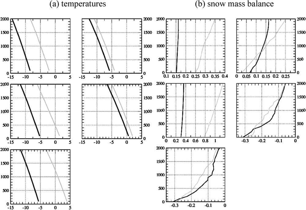
Summer temperatures (in °C) and mean annual snow mass balance (mm/day) over the Fennoscandian ice-sheet in the cold (black line) and warm (grey line) phases of a Dansgaard–Oeschger cycle as simulated by CLIMBER2.3. The results are given as a function of altitude. Top row: 70–80°N latitude band, central row: 60–70°N, bottom row: 50–60°N. Left-hand-side column: western Europe, right-hand-side column: central Europe.
Températures estivales (en °C) et bilan annuel net de neige (accumulation moins ablation, en mm/jour) sur la calotte fennoscandinave pendant la phase froide (en noir) et chaude (en gris) d'un cycle de Dansgaard–Oeschger, tel que simulé par CLIMBER2.3. Les résultats sont donnés en fonction de l'altitude. Ligne supérieure : latitudes comprises entre 70° et 80°N, ligne centrale : latitudes comprises entre 60 et 70°N, ligne inférieure : latitudes comprises entre 50 et 60°N. Colonne de gauche : Europe de l'Ouest, colonne de droite : Europe centrale.
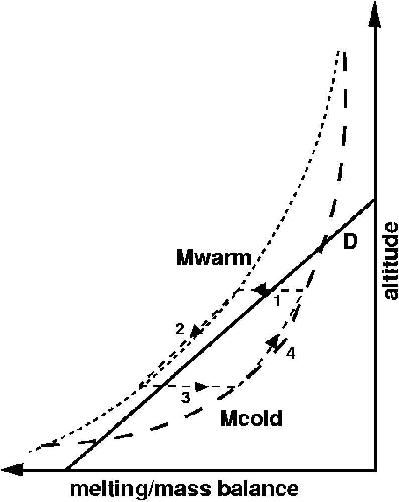
Proposed mechanism for a climate–ice-sheet system oscillation. 1. Because of a reduced fresh water delivery from the ice-sheet, the ocean switches to its most active mode, which corresponds to the warm state. 2. Ice-sheet melting increases, ice-sheet mass balance is negative because the melting Mwarm is larger than the restoring term D. The ice-sheet altitude decreases, which causes the melting and fresh water delivery to the ocean to be larger and larger. 3. Due to this increased fresh water flux to the ocean, the ocean circulation switches to its less active mode, i.e. the cold mode. 4. Ice-sheet melting decreases, ice-sheet mass balance becomes positive, the ice-sheet altitude increases, causing the melting to decrease more and more. We are then back to 1.
Mécanisme proposé pour une oscillation du système climat–calotte glaciaire. 1. Une réduction du flux d'eau douce arrivant à l'océan depuis la calotte entraîne une bascule de l'océan vers son mode actif (en termes de circulation profonde à grande échelle), qui correspond à un mode climatique chaud. 2. Dans ce mode chaud, le terme de fonte Mwarm est plus grand que le terme de rappel (ou terme dynamique) D. En conséquence, l'altitude de la calotte diminue, le terme de fonte devient de plus en plus grand, de même que le flux d'eau douce vers l'océan. 3. Celui-ci finit par faire basculer l'océan vers son mode le moins actif, c'est-à-dire que le système climatique bascule vers son mode froid. 4. Dans ce mode, le terme de fonte Mcold est inférieur au terme de rappel D et l'altitude de la calotte augmente, jusqu'à ce que s'opère une nouvelle bascule vers le mode chaud, comme décrit en 1.
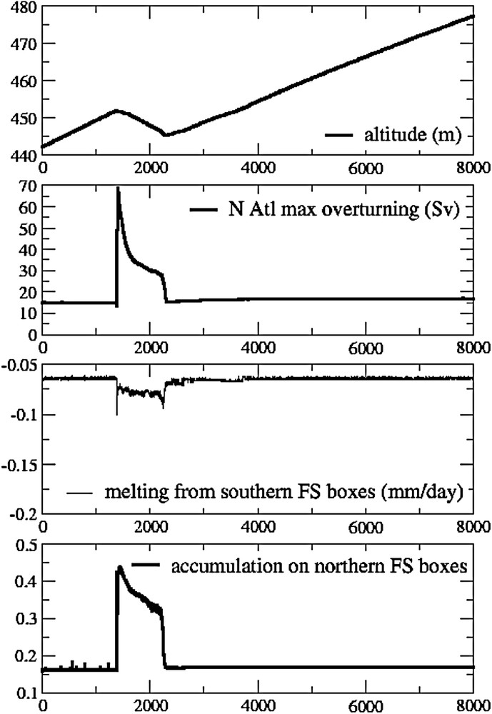
Coupling CLIMBER and the southern edge of the Fennoscandian ice-sheet: (top) altitude of the southern boxes of the Fennoscandian ice-sheet; (second from top) strength of the North Atlantic thermohaline circulation; (third from top) melting from the southern Fennoscandian boxes; (bottom) accumulation on the northern Fennoscandian boxes (mm/day).
Résultat du couplage entre CLIMBER et la partie sud de la calotte fennoscandinave : (en haut) altitude des cellules sud de la calotte ; (2e ligne) intensité de la circulation thermohaline nord-atlantique ; (3e ligne) fonte des cellules sud de la calotte ; (en bas) accumulation sur les cellules nord de la calotte fennoscandinave (mm/jour).
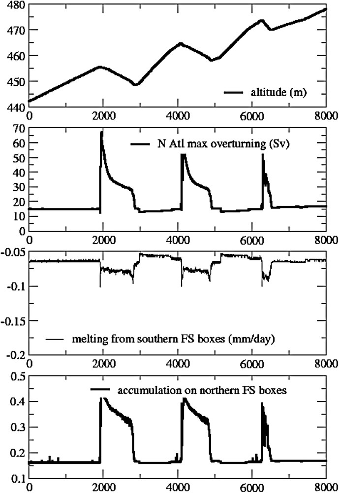
Same as Fig. 3, but the excess mass balance on the northern Fennoscandian ice-sheet is redirected to the North-Atlantic ocean with a delay of 1000 years. The systems switches three times to its warm mode, each time for a smaller duration.
Comme pour la Fig. 3, mais l'excès d'accumulation sur les cellules nord de la calotte fennoscandinave est redirigé vers l'océan Atlantique nord avec un retard de 1000 ans. Le système bascule trois fois vers son mode chaud, chaque fois pour une durée plus courte.
1 Introduction
The Dansgaard–Oeschger events identified and described in Greenland ice-cores [2] have been the focus of many studies, which have revealed that these abrupt switches to a warm state within the glacial period of Marine Isotope Stage 3 can be associated to climatic signals in many locations outside Greenland (see [1,3,6,9] for recent reviews). On the other hand, modelling studies (reviewed in [7]) have investigated several hypotheses that could explain these climatic changes that occur on the timescale of a few decades and last for a few centuries, with a period of ca. 1500 years. While some authors (such as [4]) essentially see Dansgaard–Oeschger events as the response of the atmosphere–ocean system to a varying (undefined) external forcing, others have suggested that the quasi-regular alternation between warm states (the interstadials) and cold states (the stadials) was the result of instabilities within the climate system or within one or several of the main involved components of the climate system: ocean, atmosphere, northern hemisphere ice-sheets.
The present work investigates whether repetitive abrupt warmings such as the Dansgaard–Oeschger events can be modelled as instabilities of the climate-Fennoscandian ice-sheet system. Our starting point is the experiment described in [4]. In this simulation, Dansgaard–Oeschger-type events are obtained by forcing the atmosphere–ocean system as represented by the CLIMBER2.3 model (a climate model of intermediate complexity fully described in [8]) by fresh water fluxes to the North-Atlantic ocean. These fresh water fluxes, although very small (they were described as a sinusoidal of amplitude 0.03 Sv and of period 1500 years), were sufficient to make the glacial atmosphere–ocean system switch to a different state (stadial if the system was in a interstadial state and vice-versa). This is due to the sensitivity of the glacial climate system to North-Atlantic fresh water perturbations: the hysteresis of the system is much smaller than that of the present climate and therefore the switches between the different states occur for approximately the same threshold whether the system jumps from a stadial to an interstadial or from an interstadial to a stadial. This threshold is around 0 Sv. Thus, when forced by a sinusoidal signal in fresh water in the sensitive region of North Atlantic Deep Water formation, the atmosphere–ocean system as represented by CLIMBER2.3 easily switches between the warm and cold states of the glacial period, even though the forcing fluxes are small.
From this starting point, our study proceeds in three steps. Our general objective is to examine whether the climatic oscillations obtained by forcing the atmosphere–ocean CLIMBER2.3 system with periodic fresh water fluxes could result from an internal oscillation of the northern hemisphere ice-sheet–atmosphere–ocean system. The first step is then to analyse the differences in snow mass balance over the North American and the Fennoscandian ice-sheets between stadials and interstadials in the original CLIMBER2.3 experiment described in [4]. The second step is to use the results acquired from the first step to build a very simple ice-sheet model of the Fennoscandian ice-sheet, which we couple to CLIMBER2.3. The third step is then to examine whether Dansgaard–Oeschger-type oscillations can be simulated with this model.
2 Mass balance of the North American and the Fennoscandian ice-sheets in the cold and warm phases of a Dansgaard–Oeschger cycle as simulated by CLIMBER2.3
To evaluate the northern hemisphere ice-sheet mass balance as a function of the altitude of the ice-sheet within each CLIMBER2.3 grid cell, we have developed a scheme which re-computes the surface energy budget and associated variables at 15 different levels within the given CLIMBER2.3 grid cell as if the altitude of the grid cell was at each of these levels [5]. From these calculations, we obtain, amongst other variables, surface temperature vertical profiles, and vertical profiles for snow cover, snow fall, snow melt. Fig. 1(a) shows the vertical profiles (from 0 to 2000 m) of the summer temperature over each of the five grid cells covered by the Fennoscandian ice-sheet during stadials and interstadials as simulated in the original experiment described in [4]. The cold state is around 2 °C colder than the warm state over eastern Fennoscandia. The difference is larger over western Fennoscandia, reaching around 10 °C for the southernmost box. The temperature differences do not appear to be dependent on altitude. Fig. 1(b) depicts the mean annual snow mass balance (accumulation minus ablation) for the cold and warm states. The general expected behaviour of snow mass balance as a function of altitude, i.e. increasing mass balance at higher altitude/increasing melting at low altitudes is simulated by our scheme. Two behaviours appear, depending on the location of the grid cell: the two northernmost grid cells and the central grid cell of the western sector of the Fennoscandian ice-sheet undergo snow accumulation for both stadials and interstadials, with a larger accumulation for warm periods; the two grid cells at the southern edge of the ice-sheet show negative snow mass-balance for both periods and all altitudes between 0 and 2000 m, with a larger melting for warm periods. For both periods, snow melt in the southern grid cells at sea-level is around 0.3 mm/day while it decreases to less than 0.06 mm/day at 2000 m. The difference in snow melt between the cold and warm periods is mainly located between 500 and 1500 m and reaches, at most, 0.05 mm/day, i.e. ∼18 mm/year. Hereafter, these two southern boxes are defined as the southern Fennoscandian ice-sheet while the northern accumulating grid cells are defined as the northern Fennoscandian ice-sheet.
The differences in snow mass balance between stadials and interstadials for the North-American ice-sheet (not shown) are much smaller than those depicted for the Fennoscandian ice-sheet on Fig. 1. In particular, snow melting in the southernmost grid cell of the North American ice-sheet (40–50°N) is very small (∼0.01 mm/day) and is not significantly different during a warm event, compared to the cold state. Similarly, accumulation over the other grid cells is only slightly sensitive to a warm event: the mass balance decreases by 0.01 mm/day at most during a warm event on the grid boxes between 50 and 70°N and does not vary at all on the two northernmost grid cells.
The mass balance of the Fennoscandian ice-sheet is therefore much more sensitive to the climatic state, stadial or interstadial, than the North-American ice-sheet. This is not surprising given the pattern of climatic change between the stadials and interstadials simulated by CLIMBER2.3, which affects more the European side of the Atlantic ocean than the American side [4]. In the following, we build a simple model of the Fennoscandian ice-sheet to examine whether Dansgaard–Oeschger type oscillations can be the result of an instability of the coupled atmosphere–ocean-Fennoscandian ice-sheet system.
3 A mechanism for atmosphere–ocean–ice-sheet instabilities
The mechanism we propose to examine in the present work is based on the typical shape of snow mass balance for warm and cold periods, previously described for the southern edge of the Fennoscandian ice-sheet, and is illustrated on Fig. 2. We can describe the change in altitude of the southern Fennoscandian ice-sheet dz as a function of its mass balance which can be computed, in a very simple way, as follows: , where M is equal to the snow mass balance computed by CLIMBER2.3, D is a dynamical term which represents the ice mass brought from the northern part of the ice-sheet (on which the snow mass balance is always positive). Here we have taken , where is a reference altitude and τ is a characteristic relaxation time. In the present study, we have chosen to be typically higher than the southern Fennoscandian ice-sheet altitude, so that this term represents the ‘feeding’ of the southern part of the ice-sheet by its northern part.
The ice mass balance of the southern Fennoscandian ice-sheet can be visually evaluated from the schematic on Fig. 2. For interstadials, the snow mass balance Mwarm (short-dashed line) is larger than the dynamical feeding from the northern part of the ice-sheet D (continuous line), hence the altitude of the southern Fennoscandian box will be decreasing. Conversely, for a stadial, the snow mass balance Mcold (long-dashed line) is smaller than D and the southern ice-sheet altitude will be increasing. Hence, the segments 2 and 4 on the cycle presented on Fig. 2 are always followed as shown by the arrows: decreasing altitude for 2, increasing altitude for 4.
We can now describe the proposed mechanism for an oscillation with abrupt switches between stadials and interstadials, starting from segment 4, in which melting is small and the southern Fennoscandian altitude is increasing. In this state, the North-Atlantic Deep Water (NADW) formation is rather weak. As the altitude of the southern Fennoscandian ice-sheet increases, melting gets smaller and smaller. Delivery of fresh water to the adjacent ocean, the North Atlantic, is smaller and smaller, until the ocean abruptly switches to a state with a more active NADW formation. This is equivalent to switching to a warm mode and is described by segment 1. The system then follows segment 2: melting is larger than D and the altitude decreases. As the altitude decreases, melting gets larger and eventually, fresh water delivery to the North Atlantic ocean becomes large enough to significantly slow down NADW formation, hence abruptly pushing the system in a stadial mode. The system has then come back on segment 4 and the cycle can start again.
The cycle described above can work only if the variations of the fresh water fluxes to the ocean are large enough for the ocean to switch from one state to the other. From the study described in [4], we know that for the glacial system, the thresholds for a switch on and a switch off of the deep ocean circulation are close to each other and close to a fresh water flux delivered to the 50–70°N Atlantic ocean equal to −0.02 Sv. The difference in snow mass balance shown on Fig. 1 is equivalent to a difference of at most 0.01 Sv in the fresh water delivered to the ocean, which is of the same order of magnitude as the fresh water flux forcing used by [4] to obtain their switches between stadials and interstadials. However, since the snow falling over Fennoscandinavia is now used by our conceptual ice-sheet instead of directly being routed to the sea, the threshold of the thermohaline circulation is slightly different from [4] and closer to zero. It is then worth testing the mechanisms described here by coupling our very simple model of the southern Fennoscandian ice-sheet to CLIMBER2.3.
4 A test for the proposed instability mechanism with a very simple ice-sheet model coupled with the atmosphere–ocean-vegetation model CLIMBER2.3
In all the experiments described in this section, we have coupled our very simple model of the southern Fennoscandian ice-sheet to the atmosphere–ocean model CLIMBER2.3. The melting from the ice-sheet is always directed to the most sensitive latitudes of the North Atlantic ocean: between 50 and 70°N. To facilitate transitions between cold and warm states and compensate for the low interannual to decadal variability of the climate simulated by the model, we have also introduced some variability in the fresh water flux delivered to the ocean. This has been implemented by adding a random flux of maximum amplitude 0.05 Sv (this flux is randomly distributed between +0.05 Sv and −0.05 Sv) to the fresh water flux computed from the ice-sheet mass balance.
4.1 A first attempt: coupling the southern edge of the Fennoscandian ice-sheet to CLIMBER2.3
In the applications described hereafter, and years. Fig. 3 shows our first attempt to obtain the cycle described in the previous section. Starting from a cold state, the altitude of the southern Fennoscandian ice-sheet (top plot) increases. It is difficult to distinguish the decrease in southern Fennoscandian melting on the third plot but after ∼1200 years, the system switches to its warm mode, as shown by the strength of the North-Atlantic thermohaline circulation (second plot). The altitude of the southern Fennoscandian ice-sheet then starts to decrease, melting is increased, until the system comes back to a cold mode ∼2200 years after the beginning of the simulation. From then on, the altitude increases but the system never switches to a warm mode again. Coupling the southern Fennoscandian ice-sheet to the atmosphere–ocean of CLIMBER2.3 is therefore not sufficient to obtain several stadial-interstadial cycles.
The problem comes from the fact that the cold mode reached after 2200 years of simulation is not exactly the same as the cold mode the simulation started with. The value of the North-Atlantic meridional overturning is slightly larger and the sea-ice edge has moved northward by one oceanic grid cell (2.5°). This situation, although not very different from the initial one, is characterised by a different sensitivity to fresh water fluxes. The decrease in southern Fennoscandian ice-sheet mass balance never gets large enough to trigger another switch to a warm mode, even though we have implemented a variability in the fresh water fluxes given to the North-Atlantic ocean.
4.2 Second attempt: closing the fresh water budget
The lowest plot on Fig. 3 shows the snow mass balance on the northern Fennoscandian ice-sheet during the run. As expected from the mass balance shown on Fig. 1, accumulation is much larger during the interstadial. This excess of ice should eventually reach the ocean and therefore represents a potentially large perturbation of the fresh water balance of the North-Atlantic surface. Our second attempt is based on the use of this fresh water reservoir to make the system switch to the exact cold mode as the initial state. Keeping the approach simple, we have simply redirected the excess northern Fennoscandian mass balance to the North Atlantic ocean with a delay of 1000 years. This corresponds to an additional fresh water flux of 0.02 Sv at maximum into the North Atlantic. The results of this new simple model of the Fennoscandian ice-sheet coupled to CLIMBER2.3 are shown on Fig. 4. This time, the atmosphere–ocean-Fennoscandian ice-sheet system switches back to its initial cold mode, as shown by the small decreasing step following its return to a cold mode (for instance just before year 2500 of the simulation). The system can then switch back to its warm mode and describes three cycles which are of smaller and smaller amplitude. This is reminiscent of the actual Dansgaard–Oeschger events, whose amplitude and duration decrease until a Heinrich event starts a new Bond cycle.
5 Conclusion and perspectives
The experiments described above show that it is possible to build a very simple Fennoscandian ice-sheet model which, once coupled to the climate model of intermediate complexity CLIMBER2.3, gives rise to oscillations of the glacial atmosphere–ocean-Fennoscandian ice-sheet between stadials and interstadials. However, it is important to underline the limitations of our approach. As shown by Figs. 3 and 4, the variations of the southern Fennoscandian fresh water flux to the ocean once in a given mode (either cold or warm) are extremely small. Additional experiments show that they are primordial to start the cycles, but this relative lack of sensitivity of the southern Fennoscandian ice-sheet w.r.t. altitude makes our model very fragile. The ocean needs to be very close to the threshold in which it switches from an active to a sluggish thermohaline circulation and vice versa for the mechanism to work. Other sources of fresh water flux fluctuation to the North Atlantic, such as the behaviour of the Laurentide ice-sheet, will have to be included in our model.
Acknowledgements
We wish to thank PIK for providing the CLIMBER2.3 model. MK is funded by CNRS, DP by CEA. This work was supported by French PNEDC project VAGALAM. This is LSCE contribution number 1789.