

Version française abrégée
En comparaison des événements abrupts qui ont ponctué le dernier âge glaciaire et qui ont eu des fluctuations de température de plus de 10 °C en un siècle au Groenland, l'interglaciaire actuel semble relativement stable dans le secteur de l'Atlantique nord [8,17], si l'on excepte l'événement rapide survenu il y a 8200 ans [11]. Cet interglaciaire est caractérisé par une variabilité significative dans des échelles de temps décennales à millénaires. Les dernières grandes variations climatiques du dernier millénaire en Europe ont été les périodes de l'optimum climatique médiéval (situé aux alentours de 1000–1200 AD) et le petit âge de glace, dont la durée s'est étendue de 1500 à 1850 [6] – les dates dépendant du type de données et de la région considérée [19]. Ces deux périodes sont bien documentées en Europe de l'Ouest, avec des enregistrements paléoclimatiques incluant les étendues de glaciers, l'épaisseur de cernes d'arbres et d'anciens relevés météorologiques, mais leur amplitude est d'un ordre de grandeur inférieur à celle de l'événement d'il y a 8200 ans. Cependant, ces changements climatiques ont eu des répercussions importantes sur la société, impliquant famines, maladies et bouleversements sociaux [22,23], à cause d'étés pourris successifs ou de précipitations intenses qui ont détruit les récoltes.
De telles observations de la vulnérabilité de la société suggèrent que des variations intra-saisonnières (ou brèves) peuvent avoir un impact plus grand sur la société que l'augmentation séculaire de la température. Ceci motive l'étude de la variabilité climatique naturelle au cours des derniers siècles, à partir des observations et de simulations numériques. L'étude de la variabilité passée nous permettra de comparer ses propriétés avec celles de la variabilité présente et de tester si les perturbations engendrées par les gaz à effet de serre ont aussi un impact sur des phénomènes climatiques à courte vie.
Les reconstructions de températures de l'hémisphère nord de Mann et al. [25] ont montré comment ces deux épisodes climatiques, l'optimum médiéval et le petit âge de glace, s'insèrent dans une perspective millénaire, et ont mis en évidence le réchauffement exceptionnel du XXe siècle. Luterbacher et al. [24] ont utilisé un mélange de données historiques, de données instrumentales et de cernes d'arbres pour obtenir une reconstruction mensuelle des températures sur l'Europe de l'Ouest depuis le XVe siècle. Leur étude souligne les différences saisonnières et régionales du changement climatique et donc la nécessité de multiplier les sources d'observations pour des reconstructions de la variabilité fiables et pertinentes.
Pour obtenir de longues séries de température, antérieures au XVIIe siècle, il est nécessaire d'utiliser des données proxy, c'est-à-dire des indicateurs biologiques ou géochimiques des variations climatiques [6,18]. Par exemple, une saison chaude favorise la croissance des cernes d'arbres, si bien que d'épais cernes peuvent être expliqués par de fortes températures. Donc les données proxys utilisées pour reconstruire le climat du dernier millénaire comprennent (i) les épaisseurs de cernes d'arbres, (ii) les analyses isotopiques de sédiments lacustres, anneaux d'arbres et coraux, (iii) les températures de puits de forage et (iv) les chroniques historiques [5,18]. Chacun de ces indicateurs présente une dépendance au climat qui peut être inversée pour produire, de manière au moins qualitative, les variations climatiques passées.
Le laboratoire des sciences du climat et de l'environnement (LSCE) de Gif-sur-Yvette est impliqué dans plusieurs aspects de l'étude du climat de l'Holocène, dont les reconstructions climatiques à partir de données géochimiques et historiques ainsi que la simulation du climat. Cet article illustre les efforts produits au LSCE pour reconstruire les températures et la circulation atmosphérique passées depuis le petit âge de glace.
Nous aborderons dans la Section 2 les grandes caractéristiques des fluctuations de la circulation atmosphérique des moyennes latitudes de l'hémisphère nord. Autour de la zone de l'Atlantique nord (environ 30°N à 70°N et 80°W à 30°E), la circulation atmosphérique est dominée par l'oscillation nord-atlantique (NAO), qui est la modulation de la circulation zonale par le dipôle de pression entre l'anticyclone des Açores et la dépression islandaise [13,37]. Dans sa phase positive, la circulation transporte chaleur et humidité vers la Scandinavie, tandis que le Sud de l'Europe est sec. Dans sa phase négative, l'humidité arrive sur le Sud de l'Europe, qui connaît des hivers plus froids. L'intensité de cette oscillation est généralement mesurée par l'indice NAO, qui est la différence de pression normalisée entre Ponta Delgada aux Açores et Reykjavik en Islande [13,31]. Les grandes caractéristiques de la circulation atmosphérique ont été établies à partir d'observations de pression de surface [32,34] effectuées en Europe depuis 1845. Un prétraitement d'homogénéisation a été effectué sur ces données, afin d'éliminer les sauts et dérives liés à des changements instrumentaux ou de sites de mesure [33]. Des méthodes statistiques élémentaires [31,32,38] ont été employées pour dégager les caractéristiques dominantes de la circulation atmosphérique observée à travers ces données (Fig. 1). Cette décomposition montre l'importance des modes d'une circulation zonale (liée à la NAO) et d'une circulation méridionale (du nord vers le sud). L'impact de la circulation liée à l'oscillation nord-atlantique [13,14,31,37] sur les conditions de surface a été évalué en calculant la corrélation, pour chaque point de grille, entre l'indice NAO et la température de surface observée depuis 1950 (Fig. 2, [32]). Les zones d'influence de la NAO ont évolué dans le temps, si bien qu'il est crucial de bien choisir les sites de reconstruction de l'indice NAO, afin qu'ils soient toujours sensibles à la circulation zonale [32].
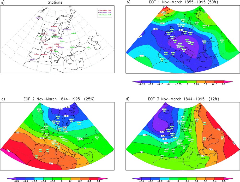
Patterns of surface pressure variability from 51 European weather stations from 1845 to 1995. (a) Location of the weather stations. Stations in red have data before 1800; stations in purple have data before 1825; stations in green have data before 1845. (b) EOF 1 of the sea-level pressure (SLP) monthly data for the extended winter (November through March). (c) EOF 2 of the SLP data expressing zonal circulation. (d) EOF 3 of the SLP data expressing meridional circulation.
Modes de variabilité de la pression de surface à partir de 51 stations météorologiques européennes de 1845 à 1995. (a) Emplacement des stations météorologiques. Les stations en rouge possèdent des données d'avant 1800 ; les stations en violet ont des données d'avant 1825 ; les stations en vert présentent des données d'avant 1845. (b) EOF 1 de la pression au niveau de la mer (SLP) des données mensuelles pour la saison froide de l'hémisphère nord (novembre à mars). (c) EOF 2 des données de SLP, représentant la circulation zonale. (d) EOF 3 des données de SLP représentant la circulation méridionale. Masquer
Modes de variabilité de la pression de surface à partir de 51 stations météorologiques européennes de 1845 à 1995. (a) Emplacement des stations météorologiques. Les stations en rouge possèdent des données d'avant 1800 ; les stations en violet ont des ... Lire la suite
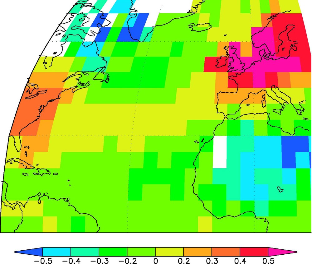
Point correlation between the NAO index and surface temperature over the North Atlantic in the winter season.
Corrélation par point de grille entre l'indice NAO et la température de surface sur l'Atlantique nord, pendant l'hiver.
Dans la Section 3, nous exposerons des résultats sur des reconstructions de précipitation, température et un indice de sécheresse en France, à partir de chroniques de dates de vendanges [7] et d'analyses isotopiques dans la cellulose de cernes d'arbres [26] (Fig. 3). La digitalisation des relevés anciens de précipitation de l'Observatoire de Paris, a montré un important changement du cycle saisonnier des précipitations à Paris entre le petit âge de glace et maintenant [30]. Slonosky [30] a montré la forte saisonnalité des précipitations à Paris entre 1750 et 1850, avec pratiquement deux fois plus de précipitations en été qu'en hiver. Au cours du XXe siècle, cette saisonnalité s'est fortement atténuée, avec des précipitations uniformément réparties dans l'année. Cette analyse montre également la dépendance du cycle saisonnier aux variations climatiques séculaires.
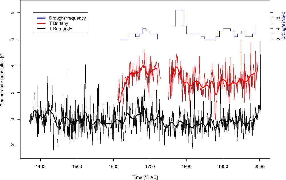
Top curve: drought index in Brittany from isotopic analyses of cellulose in tree rings; middle curve: July temperature anomaly reconstruction in Brittany, shifted by +2 °C (to enhance readability); bottom curve: warm-season temperature reconstruction from harvest dates in Burgundy. The thick lines (middle and bottom curves) represent 20-year moving average filters.
Courbe du haut : indice de sécheresse en Bretagne, calculé à partir d'analyses isotopiques de la cellulose de cernes d'arbres ; courbe du milieu : reconstruction des anomalies de température de juillet par rapport à la normale (1960–1980) et décalées de +2 °C (pour améliorer la lecture de la figure) ; courbe du bas : reconstruction des anomalies de température (par rapport à la normale 1960–1980) de la saison chaude en Bourgogne à partir de dates de vendanges depuis 1370. Les lignes épaisses (courbes du milieu et du bas) représentent des filtres à 20 ans. Masquer
Courbe du haut : indice de sécheresse en Bretagne, calculé à partir d'analyses isotopiques de la cellulose de cernes d'arbres ; courbe du milieu : reconstruction des anomalies de température de juillet par rapport à la normale (1960–1980) et décalées ... Lire la suite
Un modèle de phénologie de la vigne a été mis au point pour le cépage du pinot noir en Bourgogne. Ce modèle permet de relier les étapes clefs de la maturation du grain avec les températures de la saison chaude en France (avril à août). Une des étapes les plus importantes est la véraison du grain, c'est-à-dire le moment où il change de couleur, de vert à noir ou jaune. En Bourgogne, la vendange est décrétée une trentaine de jours après la véraison. Une fois ce modèle calibré sur le présent, il a été inversé afin de reconstruire les températures d'été en Bourgogne, depuis 1370, à partir des dates de vendanges collectées par Le Roy Ladurie [21]. La reconstruction de température est très semblable aux températures observées en Bourgogne ou à Paris depuis le XVIIIe siècle et ne présente pas de tendances « non climatiques », ce qui suggère que les effets historiques, économiques et biologiques sont assez faibles sur l'ensemble de la série. Cette série de températures montre une entrée dans une phase froide du petit âge de glace vers 1430, et un deuxième refroidissement important vers 1630, marquant la deuxième phase de cet épisode froid en Europe (Fig. 3). La caractéristique frappante de cette série est le record de température réalisé en 2003, avec un écart de +5,86 °C par rapport à la normale : c'est l'été le plus chaud enregistré en Bourgogne [7].
Des mesures isotopiques (
Il est probable que la variation climatique du petit âge de glace soit une combinaison de ces effets. Des efforts de modélisation numérique sont en cours au LSCE et à l'institut Pierre-Simon-Laplace pour comprendre les effets de chacun de ces mécanismes sur le climat de surface et ses modes de variabilité.
1 Introduction
Compared to the abrupt events punctuating the last glacial period that reached fluctuations of more than 10 °C in Greenland within a century, the current interglacial period seems much more stable in the North Atlantic sector [8,17], apart of one rapid event 8200 years ago [11] It is however characterised by a significant variability in the decadal to millennial time scale, with the last of these millennial scale variations occurring in Europe during the so-called Medieval Warm Period (MWP: circa 1000–1200 AD) and the Little Ice Age (LIA) whose time frame is approximately 1500–1850 AD) [5] depending on the regions and proxy that are considered [19]. These two periods have been documented in Western Europe from various palaeoclimatic records including glacier extent, tree ring widths, and early instrumental records, but their amplitude did not reach the glacial events or the one 8200 years before present. Yet, such changes have had important impacts on society, implying famines, diseases and social upheavals [22], due to repeated cold summers or heavy precipitations that destroyed crops.
Such observations of society vulnerability suggest that intra-seasonal (or brief) variations can have a larger impact than a secular increase of temperature, depending on the magnitude of the event. This motivates the study of natural climate ‘fast’ variability for the last centuries, from data or simulations, and the relation between secular trends and such events. An assessment of past variability allows us to compare its features with the present variability and test whether the recent perturbation induced by greenhouse gases also has an impact on short lived phenomena.
The northern hemisphere temperature reconstruction of Mann et al. [25] shows those climatic episodes in a millennial perspective and emphasizes the warming of the 20th century as being exceptional. Luterbacher et al. [24] used a blend of historical and instrumental data to obtain a detailed monthly temperature reconstruction over Western Europe since the 15th century. Their study emphasizes the seasonal and regional differences of climatic changes and hence the necessity to multiply the sources of observations for reliable and sensible reconstructions.
Temperature and pressure variations have been measured since the mid-17th century, when the thermometer and the barometer were invented. Although sparse in space and with rather primitive instruments, the measurements were performed by the top scientists of those times (including Gallileo, Cassini, Maraldi...). Most systematic measurements were local and came from personal initiatives (like Morin). The first operational meteorological network was developed by Le Verrier (astronomer at the Paris Observatory and counsellor of Napoleon III) in 1875 and covered an area extending form Western Europe to Turkey. This network gathered daily pressure and temperature readings from telegraphic communications. But it was rapidly superseded by the development of the Meteorological Office in England.
Longer temperature estimates have to rely on proxy data, i.e. biological or geochemical indicators of climate variations. For instance, a warm and/or wet season favours the growth of tree rings, so that thick rings can be explained by high temperatures. The dependence of tree ring data to temperature and hydrology highly depends on the location; it is important to calibrate it for each climatic region. The proxy data that are used for climate reconstructions of the past millennium include (i) tree-ring widths, (ii) isotopic measurements from lake sediments, tree rings, benthic corals, (iii) borehole temperatures, and (iv) historical chronicles. Each of these types of proxies has a climate dependence that can be inverted to provide at least qualitative regional temperature variations.
The ‘Laboratoire des sciences du climat et de l'environnement’ (LSCE, Gif-sur-Yvette, France) is involved in various aspects of climate studies during the Holocene, including climate reconstructions using historical and geochemical proxy data and model simulation. This paper samples the efforts held at LSCE in the reconstruction of past temperatures and atmospheric circulation over Western Europe since the Little Ice Age. We first summarize the work on past atmospheric circulation reconstruction and its connection with surface temperature. Then results obtained from various proxy data sources are explained. Finally, mechanisms responsible for climate variations since the Little Ice Age are discussed.
2 The past atmospheric circulation
2.1 Defining the North Atlantic Oscillation
The principal climate mode of variability around the extratropics is the North Atlantic Oscillation (NAO), which controls the strength and direction of the westerlies that sweep North Atlantic. The NAO is the modulation of the pressure dipole between the Azores anticyclone and the Icelandic depression. In its positive phase, the atmospheric circulation is conveyed by more vigorous westerlies and blows mainly to from America to Scandinavia, where it brings ocean moisture; the Mediterranean region is then drier and warmer than normal. In its negative phase, the westerlies are weak and the circulation brings moist air over southern Europe.
It is generally measured by the so-called NAO index, which is the normalised monthly pressure difference between the Azores and Iceland. The relevance of the NAO index can be explained by the geostrophic wind, emerging from the equilibrium between Coriolis and pressure forces in the extra-tropics. The horizontal geostrophic wind is proportional to the pressure gradient, according to the equation:
| (1) |
The NAO is connected to the Arctic Oscillation (AO), which reflects the principal mode of variability of the northern hemisphere atmospheric circulation [36]. The AO corresponds to the modulation of a zonally symmetric circulation blowing to the east, so the NAO can be viewed as a projection of the AO over the North Atlantic sector.
2.2 Variability of the NAO since 1850
Surface pressure data from 51 European meteorological stations were used to determine the patterns of atmospheric circulation from 1755 to 1871 [18]. The data were homogenised using an iterative procedure of multiple comparisons and adjustments [33]. The homogenisation exercise was necessary in order to remove spurious variations in the surface pressure records caused by station relocations (including changes in the height of the barometer), instrument changes, changes in observing practices and methods of calculating monthly means, and other such non-climatic variations. The magnitude of non-climatic inhomogeneities can be as large as, or even larger than, climatic signals, and so a homogenisation exercise is an essential preliminary step to any data analysis. Periods identified as inhomogeneous were corrected on a monthly basis to a standard mean period (usually taken as 1980–1995), using the assumption of continuity of the mass of air over long periods of time.
In order to extract the dominating modes of the atmospheric circulation, empirical orthogonal function (EOF) analysis [38] of the surface pressure was performed on the stations in the pressure dataset that gathers continuous measurements made since 1844. The EOF analyses were performed on monthly winter data (Fig. 1). The first EOF explains the overall tendency of the pressure field over the domain to be above or below average, and is linked to the general synoptic character of a given month, dominated by high- or low-pressure synoptic systems. This EOF accounts for 50% of the variance in the surface pressure field. The second EOF (25% of variance) shows a dipole pattern, with loadings in the northern half of the domain of opposite sign to those in the southern half, and appears to be linked to an anomalous zonal flow; this pattern implies enhanced westerly flow in the positive phase and weak westerly or easterly flow in the negative phase. The third EOF pattern (3% of the variance) appears to be a pattern associated with anomalous (anti)cyclonic (blocking/enhanced cyclonicity) flow over the eastern Atlantic and meridional flow over Europe.
The principal components (PCs) were calculated by projecting the EOF matrix onto the normalised data. PC 2 is considered here as an index of large-scale zonal flow over the eastern Atlantic and Europe, while PC 3 is considered as an index of meridional flow over Europe and the eastern Atlantic. The correlation between the NAO and zonal flow indices like PC 2 was shown [34] to vary from between 0.7 in winter to only 0.2 in summer. However, a more meridional circulation type depicted by EOF 3 was found to be correlated with the NAO with a value of about 0.5 throughout the year. The quadruple pole correlation pattern between surface temperature and the NAO can be attributed to enhanced cyclonic flow over the northern North Atlantic and enhanced anticyclonic flow over the subtropical North Atlantic, advecting warm oceanic air over Europe and southeastern North America, while anomalously cool air is transported over the Labrador Sea, Greenland and northwest Africa.
2.3 Temperature impact of the NAO
The influence of the NAO on surface temperature can be determined from the monthly gridded near surface temperature data set for 1856–2000 of the Climatic Research Unit, Norwich, UK. The dataset is a blend of land surface temperature and sea surface temperature [18,27]. The temperature values are given as departures from the 1961–1990 mean for each
A correlation map between winter temperature anomalies and the NAO index over the North Atlantic and surrounding land-masses shows four main regions of correlation (Fig. 2): positive correlations over Europe and southeastern North America, and negative correlations over Greenland and the Labrador Sea region and over northwestern Africa [14,20,31]. The influence of the NAO on North Atlantic surface temperature captures the combined effect of the Icelandic Low influencing the advection of cold air over Greenland and warm air over Europe, and the Azores High controlling warm air advection over the southwestern North Atlantic and cold air advection over Africa.
2.4 Precipitation regimes
Precipitation measurements taken at the Paris Observatory from the 1680s to the 1750s were digitised by Slonosky [30]. These values were blended with modern data until 2001. The most striking change in the precipitation patterns over the past 300 years is the change in seasonal distribution. In the late 17th and 18th centuries, summer precipitation accounted for 60% of the yearly total, changing to a uniform seasonal distribution in the 20th century. Winter precipitation has increased by 24 mm per century, while summer precipitation increased by 4 mm per century. The winter of 2000/2001 was the wettest of the past three centuries; the year 2000 recorded the largest amount of precipitation since observations began.
These changes in precipitation may be related to changes in atmospheric circulation. Since pressure data in Gibraltar or Reykjavik do not go before 1825, an index of European zonal wind was calculated as the difference in normalized pressure between Paris and London, which have a longer time span. This index is well correlated in winter with the usual NAO index and showed more frequent reversals in the zonal flow, with ensuing dry, easterly and northeasterly winds over northern France around the turn of the 18th century [34]. Several authors have commented on the more continental climate of the 17th and 18th centuries in Europe, compared to a milder, more maritime climate in the 20th century [15]. However, correlations between precipitation at Paris and the NAO index are not significant [34], which suggests that the precipitation long-term variations are not controlled by the zonal flow captured by the NAO index. Indeed, the Paris precipitation seems to be more highly correlated with a circulation pattern depicting large-scale cyclones and anti-cyclones passing through central western Europe (the third EOF of surface pressure over Europe 1844–1995, Fig. 1), with significant correlation coefficients ranging from 0.67 in February to 0.44 in August. This inference is corroborated by the analysis of Yiou and Nogaj [39], who computed the association between daily weather regimes and the occurrence of precipitation extremes. They found that the probability of observing drier winters was increased with more frequent meridional types of circulation, like the ‘Scandinavian blocking’. It is thus probable that the NAO circulation, with its zonal component, was less frequent during the Little Ice Age than it is at present.
3 New climate proxy reconstructions
3.1 Isotope data from tree rings
A new palaeoclimatic reconstruction for western France was obtained from tree-ring cellulose stable isotopes [26,28]. Living trees from the Rennes Forest and beams from two ancient buildings in Rennes city have been combined to cover the past four centuries with a gap from 1730 to 1750. The cellulose
The decadal winter/spring NAO indices exhibit common decadal fluctuations with the
A crude method to define extreme years is to identify years when the water stress deviates from the mean value by one or two standard deviations, for a Gaussian variable [26]. Hence an extreme year is characterized by an annual parameter exceeding the 1951–1996 mean by more than one standard deviation (which means a reconstructed water stress lower than 0.51), corresponding to 15% of the samples.
Fig. 3 shows that the occurrence of extreme dry years (measured by the number of years between successive droughts) identified from the Rennes ring isotopic composition systematically increases during local warm and dry periods (e.g., in the 20-year periods centred around 1680, 1770–1780, 1900–1910, 1950 and the 1990s). In particular, the well-known droughts of the 1780s, which had led to large-scale famines [21] are captured. With this definition, the median drought recurrence is four years and the mean drought recurrence 6.8 years. The relationship between these extreme dry years and the atmospheric circulation dynamics still remains to be understood.
When the full record is considered, the mean reconstructed summer temperature is 18.2 °C and extreme dry years occur at a frequency of 2.5 per 20 years. In order to relate the mean climatic condition to the frequency of extreme events, 35 20-year-long subsets of the climate record (e.g., from 1980 to 1960, 1970 to 1950 and so on) were extracted. For each subset, both the mean bidecadal reconstructed temperature and the number of extreme dry years as defined previously were calculated. These subsets were classified into two groups: ‘cool periods’ with a lower than average mean summer temperature, and ‘warm periods’ with summer temperature above the full record average. The mean bidecadal temperature and frequency of extreme dry years for the cool versus the warm periods can hence be evaluated. Thus, cool periods correspond to a mean summer temperature of
3.2 Harvest dates
Harvest dates have provided useful information since their systematic record in France and offer a potential for a global cover of western Europe since the Middle Age. In France, harvest dates (minimum authorized harvest date) have been decreed by regional authorities at least since the early 13th century in Burgundy (e.g., Beaune municipal archives), and have been carefully registered in parochial archives and later in municipal archives. This information is thus unaltered through time and the chronology is perfectly established. Vine domestication started thousands of years ago and propagated vegetatively. Some cultivars (vine varieties) originated in the regions in which they are still grown, and others were introduced by traders or conquerors, and a few produced by controlled cross breeding since the mid-1800s. Vine development annual cycle strongly depends on climate conditions – especially temperature, with earlier harvest dates occurring during warm spring and summer years (
Angot [2] started to collect historical data on harvest dates and was the first to connect them to climate fluctuations, although qualitatively. Le Roy Ladurie [21] investigated the impact of climate variations on society since the Middle Age. He particularly focussed on records of harvest dates in France and connected the large anomalies with famines and diseases that struck France. Souriau and Yiou [35] used Le Roy Ladurie's series to investigate the impact of the NAO on the harvest dates and used their unambiguous chronology to validate NAO indices based of proxy data.
Chuine et al. [7] used Pinot noir harvest dates in Burgundy for their climate reconstruction. Pinot noir was born in Burgundy where it remained the major cultivar till today especially since Duke Philippe the Hardy decreed the destruction of Gamay, second cultivar cultivated in Burgundy, in 1395 in favour of Pinot noir, which provided a wine of better quality. Other evidences of the presence of Pinot noir in Burgundy are attested since at least the 14th century. This cultivar was thus the best candidate to trace back temperature anomalies in Burgundy since 1370. A processed-based model was devised to connect daily mean temperatures and the maturation phases of vine. This model was calibrated on recent and thorough observations of pinot noir growth, including ‘véraison’. Since harvests take place about 33 days after véraison, an inversion of the model was possible to determine an average temperature compatible with long records of harvest dates (Fig. 3).
The yearly reconstruction is significantly correlated with summer temperatures in the Burgundy part of a spatial multi-proxy reconstruction
Fig. 3 shows two early warm decadal fluctuations in the 1380s (+0.72 °C) and in the 1420s (+0.57 °C), above the 95th percentile. The warm period of the 1420s was followed by a very cold period that lasted from the mid 1430s to the end of the 1450s (−0.45 °C, under the 10th percentile). This series also shows particularly warm events, above the 90th percentile, in the 1520s and between the 1630s and the 1680s, which is also detected in the tree-ring cellulose in Brittany. These decades are as warm as the end of the 20th century. The high temperature event of 1680 was followed by a cooling culminating in the 1750s (under the 5th percentile), which was the start of a long cool period that lasted until the 1970s.
The inferred anomaly for the 2003 summer is a record event: it was +5.86 °C warmer than the reference period (1960–1989), whereas the next highest anomaly during the whole period was +4.10 °C in 1523. This confirms and refines conclusions of previous studies of the exceptional character of the 2003 summer in France.
4 Discussion and conclusion
The various high resolution proxy and instrumental records that have been explored suggest that the weather patterns and the probability of observing them changed since the Little Ice Age. Hence, since each weather regime has a well-identified signature on temperature and precipitation, a change in its occurrence can have a significant impact on the regional temperature and precipitation subannual variability, with little or no effect on a hemispheric annual mean.
The mechanisms responsible for the Little Ice Age are still debated. Physically plausible mechanisms involve increasing volcano eruption or the solar variability, ocean circulation changes, most probably a combination of these. A weakening of the thermohaline circulation would have cooled the high latitudes of the North Atlantic. Detailed measurements of
Solar forcing is an intuitive candidate to explain some of the climate variations since the LIA, because the sunspot number anomalies such as the Spöhrer and Maunder minima coincide with periods of cooling in Europe. Although the direct radiative forcing of such solar variations is very weak, it can have effects on the stratospheric chemistry, which is sensitive to irradiance. A model simulation containing stratospheric chemistry showed that there was an indirect effect of solar forcing on the atmospheric circulation [29].
Volcano eruptions eject vast quantities of dust into the troposphere and stratosphere. This dust can stay up to a couple of years in the atmosphere and hence modifies the planetary albedo and the radiation properties of the atmosphere, inducing a general surface cooling. The largest past volcanic eruptions can be recorded in polar ice cores through the chemical signature they leave in the precipitation. A statistical technique was devised to detect the impact of volcanic eruptions on temperatures [1]. This study suggests that some of the cool decades of the LIA occurred during periods of high volcanic activity.
Modelling studies have suggested that, even with a rather stable intensity of the thermohaline circulation, the characteristic time scale of ocean heat transport from north to south high latitudes could account for the observed phase lag between the warmest periods in the north and in the south [6,10].
The assessment of recent climate variations is still active, through the collection of new data, predating the invention of meteorological instruments. Careful calibration is always necessary and requires multidisciplinary approaches. Model simulations, containing the important ingredients of climate dynamics, are necessary to test different scenarios. Such experiments with coupled models have been performed over the past centuries. The main difficulties to overcome in these experiments are the determination of the initial state of the ocean and the effects of solar and volcano forcing. Since little is known on the precise condition of the ocean circulation during the Little Ice Age, idealized simulations have to be devised, with specified surface temperature anomalies and a global circulation that is a compromise between the modern one and past reconstructed surface conditions. The external forcings are estimated from cosmogenic isotope measurements in tree rings and ice cores for solar activity, or chemical contents in ice cores for volcanoes. The radiative or indirect impact of such forcings has been heuristic in most numerical experiments performed so far. In the absence of a more detailed knowledge of the forcings, ensemble simulations with varying impacts are necessary to estimate the role of such ‘external’ variations on climate. Ultimately, including ingredients such as atmospheric chemistry and a detailed history of land use will be necessary to simulate accurately the climate variations since the Little Ice Age.
Acknowledgements
It is a pleasure to thank our colleagues who contributed to the ideas of this paper: I. Chuine, V. Daux, G. Hoffmann, E. Le Roy Ladurie, P. Naveau, G. Raffalli-Delerce, V. Slonosky, A. Souriau and N. Viovy. We are grateful to A. Berger for his careful review of the manuscript.