

1 Land topography from optical stereoscopy
The construction of a high-resolution topographic map is traditionally obtained by optical stereoscopy for which the most ancient workhorse has been aerial photography where a specialized plane takes overlapping high-resolution photographs [2]. A key geometric parameter in stereoscopy is the ratio between the baseline (i.e. the separation between the points where the two images are taken), and the height from which they are taken. The overlapping sectors present typically a baseline/height ratio ranging from 0.5 to 1. The exploitation of the stereoscopic pairs was traditionally performed by analogue devices before the advent of cheaper and more powerful computers in the last 15 years. This approach for topographic mapping was adapted to the early space systems allowing, for instance, the former Soviet Union to cover most of the world's topography using an analogue film recovered after the landing of the spacecraft. Despite the extraordinary achievement of these projects, the homogeneity and absolute positioning of these maps were not satisfactory, partially due to their analogue nature.
This situation improved with the era of digital photography first implemented from space. The CCD (Charge Coupled Device) onboard SPOT satellites (numbered 1 to 5) allowed the production of stereoscopic pairs on an industrial scale, using digital comparisons based on correlations rather than analogue stereoviewers [6]. The mirrors designed to allow SPOT's access to areas off the orbital track of the satellite not only permit to revisit a given area within a time shorter than the 26-day orbital cycle of the satellite, but also to create a lateral stereoscopic effect. The usual baseline ratio is similar to the one in conventional stereoscopy (in the order of 1).
Using a single, multipurpose instrument in two passes rather than a specific stereoscopic instrument is an economic advantage, but with the drawback of acquiring the dataset at two different times. This allows the landscape to change between the data takes, lowering the quality of the correlation of the images. Another drawback becomes important in areas often covered by clouds: if the probability to obtain a cloud-free image is p, the probability to obtain two such images independently is , which can be unbearably low if p is low (e.g., 10% and 1%, respectively).
These drawbacks have been partially overcome by a new generation of instruments capable of performing aft and rear imaging for producing stereo pairs such as the HRS instrument (High-Resolution Stereoscopic) onboard SPOT 5 (launched in 2002) or the PRISM instrument onboard ALOS (launched in January 2006). HRS has covered more than 50% of the land surfaces with a vertical accuracy of about 5 m. These instruments are still subject to cloud cover and can reach a global coverage only asymptotically because they are less and less efficient as they near this goal. They typically use baseline ratios in the order of 1 (such as 0.8 for HRS).
More recently, improvements in the understanding of the frequency content of optical images as well as improvements of correlation techniques have led to new concepts for optical stereoscopy, where a very small baseline ratio (for instance 0.01), resulting in very similar images, is combined with a high-performance correlation scheme, allowing the detection of about 0.01 pixel offsets and improving the final figure of accuracy [13]. Pushing this technique to the extreme, two detectors placed at different locations in the focal plane of a single instrument could generate enough baseline to produce a stereo map. Such a configuration, implemented on SPOT 5 for another purpose, has been exploited to generate maps with 10-m vertical accuracy from single data takes, at least if the topography is strong. A topographic description produced in the same reference of an optical image improves greatly the accuracy of the localisation of the latter.
The digital era reached airborne systems as well in the 1990s, leading to more accurate topographic maps, especially when combined with high-accuracy navigation systems like GPS. However, we will not discuss further the role of airborne systems here, whether optical or their equivalent in radar technology, because these systems could not practically produce a global and homogeneous topographic map, despite existing examples of large-coverage campaigns. The advent of reliable unmanned aerial vehicles and more advanced navigation devices may change this situation in the future.
Essentially produced for mapping purposes, whether civilian or military, the high-resolution topographic mapping has a variety of scientific applications. These applications are usually in support of other primary goals. For instance, accurate topographic map were used to evaluate the secular displacement of faults [4,19] or to produce the topology of river basins [23], sometimes with spectacular results. The high-resolution topographic mapping is therefore a multidisciplinary scientific tool, which must satisfy the largest possible fraction of the science community, in terms of performance as well as in terms of accessibility. An important step in this direction has been achieved by the SRTM mission, flown in 2000, which led to a first generation of topographic map sufficiently global (covering roughly between ±60° of latitude) and accurate (about 30 m of vertical accuracy for the publicly available product, on cells) to satisfy the bulk of scientific requirements in a standard format [7,24]. This mission used the technique of radar interferometry [11] described below.
2 Land topography from radar interferometry
2.1 Principles of radar interferometry
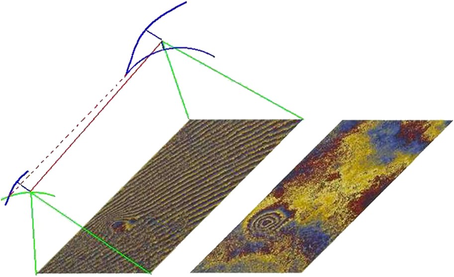
After illuminating a scene with radiowaves, a radar instrument recovers the amplitude and the phase of the returned echoes. In other terms, it produces an image made of complex numbers, each pixel being made of a real part (the amplitude times the cosine of the phase) and an imaginary part (the amplitude times the sine of the phase). In contrast with conventional imagery, the components of these complex numbers can be negative as well as positive. The amplitude image must be reconstructed through mathematical methods that rely crucially on the complex nature of the product [3,5]. At the end of this process, the resulting high-resolution image is still made of complex numbers. Most applications use only the amplitude of these numbers, which form a conventional image made of positive numbers. Interferometry aims at using the phase of a radar image to derive geometric information much like what is done with static GPS receivers in geophysical applications. The phase image produced by any imaging radar together with the amplitude image is generally discarded because it consists in random values. More precisely, the unknown layout of elementary targets within a pixel that causes the speckle effect in amplitude image results in a totally random distribution in the phase image [20]. The trick of interferometry consists of subtracting the phases between two radar images resulting in the cancellation of the phase randomness. Translated to conventional amplitude image, this results in quite similar speckle patterns. The practical procedure to achieve this is quite simple and is depicted in Fig. 1: we take two images that are, in the most general case, separated in space (that is, not acquired from exactly the same point) as well as in time (that is, acquired at different times). The difference of phase exhibited by these images can easily be predicted from the geometric layout of Fig. 1. After borrowing specialized geographic and orbital know-how (specifically for turning a topographic map into a collection of Cartesian coordinates and for determining the time and distance when the satellite is at the closest, for each set of coordinates), determining what should be the difference of phase is straightforward: the difference of the round trip distances is expressed in units of wavelengths, of which only the fractional part is retained. The theoretical difference can then be compared to the experimental one, obtained by subtracting the actual phases between the two images, provided the random part of the phases due to multiple elementary target interaction within a pixel remained the same in both images.
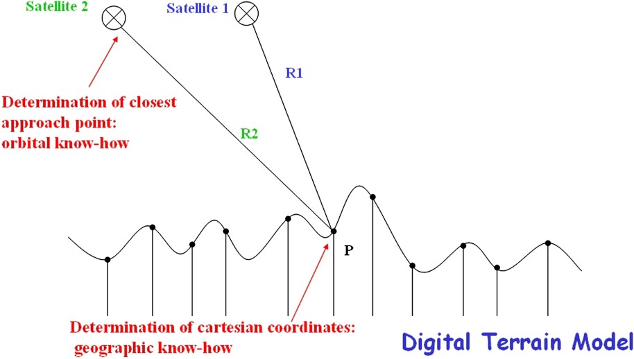
The geometry involved in radar interferometry is very simple in principle. The prediction of the difference of phase between two images requires borrowing methods from geography as well as orbitography. Assuming every parameter is known, the fractional part of the difference of the distances R1 and R2 (in round trip) expressed in wavelength units should equal the fractional cycle of phase observed experimentally by subtracting the phase of corresponding pixels in images 1 and 2.
Le principe géométrique de l'interférométrie par radar est très simple. La prédiction de la différence de phase entre deux images radar est obtenue en ayant recours à des spécialités en géographie et en orbitographie. En supposant une géométrie parfaitement connue, la partie fractionnaire de la différence des distances R1 et R2 (qui représentent des trajets aller-retour), exprimées en unités de longueur d'onde, doit être égale à la différence de phase obtenue expérimentalement par soustraction des valeurs de phase des pixels correspondants dans les images 1 et 2.
In time, this condition is quite easy to figure out: the elementary targets on the ground must not change. For instance, imaging water with any kind of time difference is hopeless and imaging an area used for agriculture requires short time intervals as the soil is periodically resurfaced. On the other hand, in desert environment, we have observed successful comparisons using images taken 10 years apart. If only part of the elementary targets remained identical within a pixel, the contribution of this part will be mixed with a noisy contribution due to the rest of the pixel, but the measurement will still be successful.
In space, the condition is more subtle and deals with the variation of the incidence angle between the images. In the most general case, we do not know the layout of elementary radar targets in the pixel. Therefore, to be meaningful, a difference of phase must give roughly the same result regardless of the actual positions of the targets in the pixel. In Fig. 2, two sets of wavefronts have been symbolically drawn in red for the first image and in green for the second. We observe from the beating pattern that the situation on the left will not work whereas the situation on the right might give a good result. For a pixel size of about 10 m across and a wavelength of a few centimetres, this condition corresponds typically to one tenth of a degree, which amounts to about a 1-km separation at most for two spacecrafts orbiting 1000 km away.
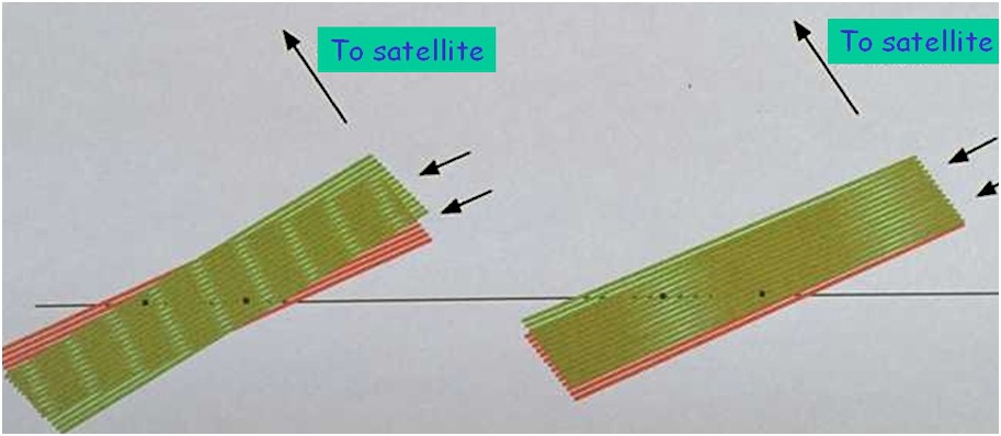
A condition for proper interferometric combination is a moderate difference of the angle of incidence between the images, so that the difference of phase does not beat within a pixel (on the left: incorrect, on the right: correct).
Une condition indispensable pour que le principe de l'interférométrie fonctionne est la limitation de la différence d'angle d'incidence entre les deux prises de vue, de sorte que la différence de phase ne puisse pas « battre » à l'intérieur d'un pixel (situation incorrecte sur la gauche et satisfaisante sur la droite).
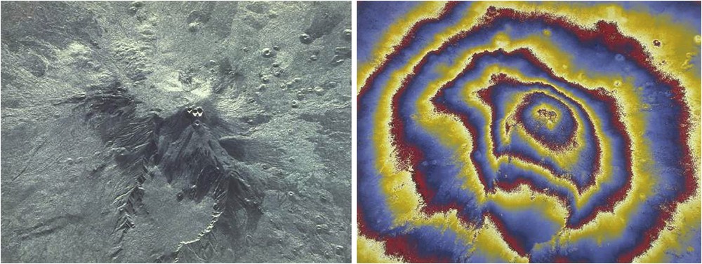
Assuming the subtraction works properly, the difference of the phases is not random anymore, as shown in Fig. 3, representing the Gulf of Aqaba (surrounded by Egypt, Israel, Jordan, and Saudi Arabia). Taking a pair of radar images, we have two conventional, amplitude images (one of them displayed in the upper left of Fig. 3) and the image of the difference of the two phase images, called interferogram (lower left), where any geometric difference between the images is recorded. A full-phase cycle, here shown as a colour cycle or fringe, amounts to one additional radar wavelength round trip from one image to the second. The radar images used in this example are separated by several months, so the result over the waters of the Gulf of Aqaba is as random, as would be the phase of a single image. The phase difference is dominated by a pattern of parallel fringes that can be eliminated. Once this is done (lower right), the result is made of two very different layers of information:
- – a topographic layer where each fringe represents a topographic contour line with, in this example, about 300-m vertical separation between contour lines;
- – a displacement layer where each fringe represents a displacement of 3 cm along the line of sight to the satellite. The 10 or so fringes visible on the west coast of the Gulf of Aqaba represent a displacement of some 30 cm caused by an earthquake that took place between the dates of acquisition of the two images.
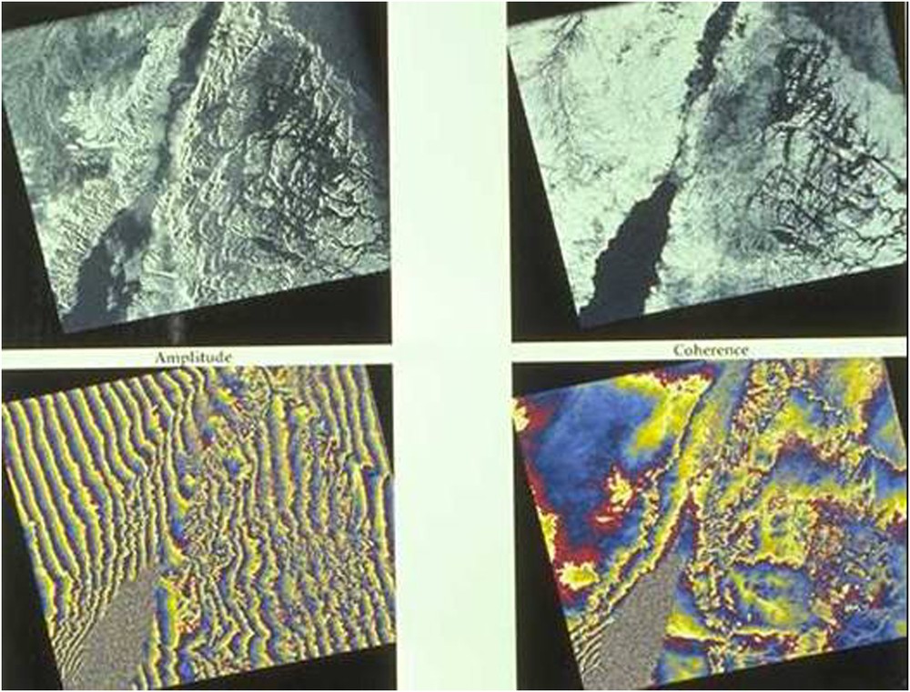
Where the right conditions are met, the phases of radar images (whose typical amplitude is shown in the upper left) can be subtracted and deliver a geometric information made of several layers (lower left) that can sometimes be separated (lower right without the ‘orbital fringes’). A coherence channel (upper right) is easily computed and maps the quality and/or reliability of the result (revealing that the Gulf of Aqaba does not show any stability over time).
Lorsque les conditions sont remplies, les phases de deux images radar (dont la partie « amplitude » de l'une apparaît en haut à gauche) peuvent être soustraites point à point et donner une information géométrique constituée de plusieurs couches (en bas à gauche) qui peuvent parfois être séparées (en bas à droite, après élimination des « franges orbitales »). Une information dite de cohérence (en haut à droite) se calcule facilement et constitue une mesure de la fiabilité du résultat, donc de la stabilité des cibles au sol (révélant ici la variabilité des surfaces d'eau du golfe d'Aquaba).
Finally, it is worth mentioning that the fringes come with a quality indicator, called coherence, which can be produced automatically with each interferogram [1]. This indicator is another image, the brightness of which quantifies the quality of the interferogram (upper right of Fig. 3). It is interesting to note that coherence detects more clearly the shoreline of the Gulf of Aqaba than the amplitude image does. For some usage, the coherence might be used as a final product, for instance is soil or vegetation studies.
2.2 Different kinds of information mixed in a single product
If we come back to our scheme, we now look at what we could learn from interferometry. If we knew everything, the theoretical prediction of the difference of phase should equal the actual phase subtraction and the interferogram would be flat. But, in our less than perfect world (Fig. 4), there are some unknowns that result in undesirable artefacts. Because the images are separated in point of view, we might commit an error in our estimation of the satellite's position, which will generate the kind of ‘orbital fringes’ that we eliminated in the previous example (between lower left and lower right of Fig. 3). Our knowledge of the topography might be inaccurate, which will alter the distances to both satellites, but with a slight difference due to the different points of view. Since the angular separation must be very small, one topographic fringe is typically created by a 10-m topographic difference for the largest separation of the satellites allowing interferometry (i.e. about 1 km), or by a 100-m topography if their separation is only 100 m. We call altitude of ambiguity the amount of elevation change that creates a topographic fringe. This way an interferogram might be regarded as a topographic map whose contour lines are separated by the altitude of ambiguity. The ambiguity results of the lines not being numbered.
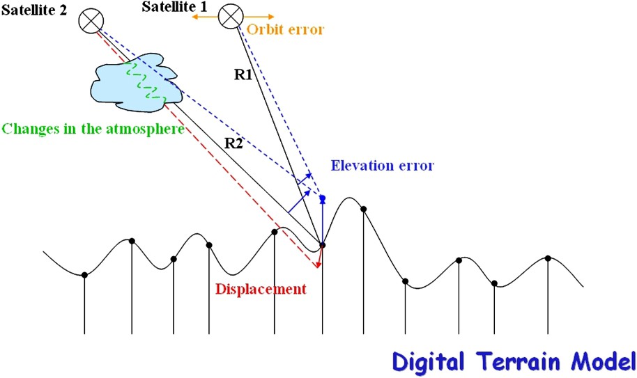
Four different kinds of information are stacked in an interferogram. Elevation errors and orbital errors do not depend on the time elapsed between image acquisitions, whereas the contributions of the atmosphere and ground displacements depend on it.
Quatre types d'informations sont « empilés » dans un interférogramme. Les erreurs de topographie et de connaissance de l'orbite ne dépendent pas du temps écoulé entre les prises de vue, contrairement aux contributions de l'atmosphère et des déplacements du sol.
If the images are separated in time, the atmosphere might alter the phase of any single image. Since radar is well known for its all-weather properties, the atmosphere will not prevent the acquisition of the image but may influence its phase, which will show up in the difference. Part of the terrain might move between the acquisitions of the images. Unlike the topography, these changes affect a single image of the pair and are directly recorded as phase changes. Therefore each fringe corresponds to a one-way displacement of half the radar wavelength in the line of sight, i.e. a few centimetres in general.
Let us summarize briefly the four layers of information provided by interferometry: first we have the contribution of trajectory uncertainty that we call orbital fringes. They can easily be eliminated by adequately changing the predicted far and near ranges according to the number of fringes we want to remove from the interferogram (Fig. 5). It is much like rotating the mirrors in an optical interferometer. Once two new trajectory tie points are defined at both ends of the image, the rest of the trajectory can be modelled because the satellite has a very predictable path (in the airborne case, the trajectory residuals would be much more difficult to cope with and some trajectory fringes would remain in the final result, unless we can reconstruct the trajectory with millimetre accuracy all along).
Geometric scheme of orbital fringe removal by trajectory correction.
Croquis indiquant le principe de l'élimination des franges orbitales par correction de la trajectoire.
The second layer is the topography, illustrated in Fig. 6 by an image of Mount Etna taken twice one day apart by a radar onboard the Space Shuttle [22]. In this example, the crew managed to fly within 20 m from the previous track, which resulted in a low topographic sensitivity because the stereoscopic effect is limited. Each fringe corresponds to a 500-m contour line. Since the signal-to-noise ratio is quite high, one 50th of a fringe might still be significant, which leads to a 10-m accuracy of the final topomap.
Radar amplitude on Mount Etna as observed by Sir-C (left) and interferogram showing the topography of Mount Etna using a second Shuttle pass one day later (right).
Amplitude de l'image radar du mont Etna, obtenue par la mission Sir-C (à gauche) et interférogramme décrivant la topographie du volcan, obtenu par combinaison avec une seconde image obtenue par la navette un jour après la première (à droite).
The 1-km rule of thumb that we gave earlier as the limit of the orbital separation is very rough. The incidence angle condition for interferometry is relaxed with a higher resolution, a longer wavelength and a larger angle of incidence, increasing the capability to obtain interferometry with satellites flying farther apart, and therefore their stereoscopic performance (characterized by a lower altitude of ambiguity). As a consequence, an L-band system (with a wavelength at around 24 cm) might be as efficient as an X-band system (with a typical wavelength of 3 cm) for high-quality Digital Terrain Model construction. This is all the more true that the time variation of elementary targets is attenuated in L band, which can penetrate the vegetation. The interferometric condition might therefore remain valid for a longer time on a given landscape if we operate in L band. This is in contrast with the traditional view of favouring X band systems for high resolution, because they are allowed a higher bandwidth.
Even a medium-resolution system such as ERS-1 can theoretically reach exceptional topographic performance. Given a proper orbital separation (i.e. a proper stereoscopic baseline) and a average signal-to-noise ratio, such a system can easily reach a 1-m vertical accuracy (for instance with 20 m contour lines and a signal-to-noise ratio high enough for 1/20th of a fringe to remain significant), but this is without considering the additional layers of information linked to the separation in time between the images.
The third layer of information constitutes a very well-known application of interferometry: the high accuracy mapping of terrain deformation such as seen with the interferogram of Fig. 7 [16]. The topographic contribution is subtracted using a terrain model and the trajectory data. What is left is the signature of several earthquakes that struck this area in southern California during the 18 months elapsed between the two acquisitions of the images. The data allow accurate observation of the deformations stacked in time. A small earthquake took place five months after the big one. Each fringe corresponds to three centimetres of deformation along the line of sight, which is half the ERS-1 radar wavelength. As for the topography, the measurement is ambiguous: we see fringes, but no value can be assigned to them, so the absolute displacement must be reconstructed by continuity, for instance starting with a point where no deformation is assumed. This operation is called ‘phase unwrapping’ [9]. The need for continuity in this operation is a strong limiting factor in some cases, for instance urban elevation modelling with buildings whose heights exceed the altitude of ambiguity.
Interferogram of Landers where various earthquakes are stacked in time.
Interférogramme de la région de Landers, où plusieurs tremblements de terre ont superposé leur marque.
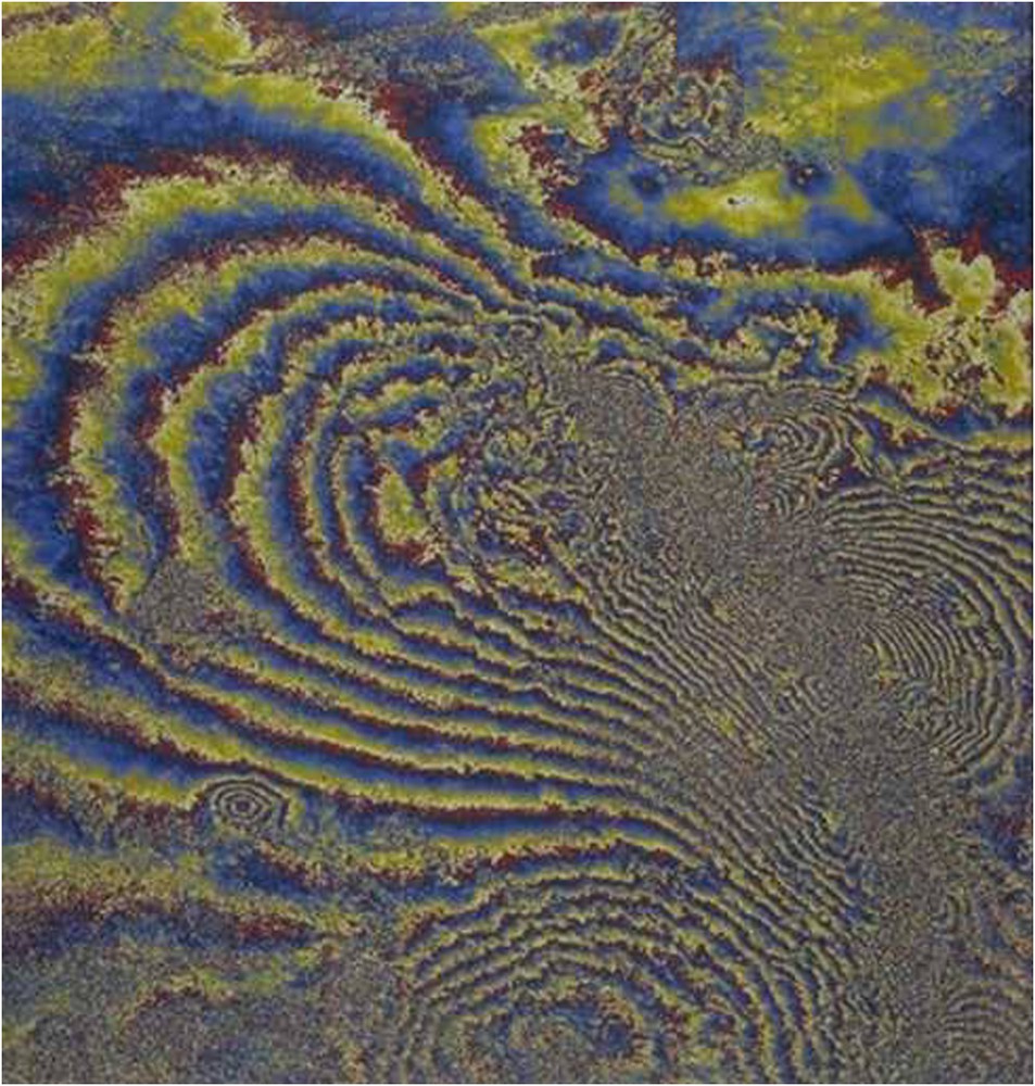
Finally, the fourth layer of information constitutes a much more worrisome problem for the topographic measurement: the contribution of the atmosphere. In Fig. 8, we have an example on the West Coast of the US, in the Blue Mountains. The topographic contribution has not been removed, but we can see these waves, which corresponds only to three millimetres crest to crest (one 20th of a wavelength). Nevertheless, with a topographic sensitivity of about 400 m, these could be misinterpreted as hills 20 m high or so. Unlike ground deformation, tropospheric, or ionospheric contributions are quite common as soon as the comparison uses images not taken at the same time [10,15,17].
Interferogram showing the effect of winds over the Blue Mountains superposed to topography.
Interférogramme montrant l'effet des vents sur les « Blue Mountains » (dans l'Est des États-Unis), qui se superpose à la signature de la topographie.
2.3 Consequences on system design
If we summarize what consequences all this has on the airborne versus spaceborne question, we have to consider two situations: the first deals with using a conventional radar in multiple passes: the satellite is very effective. The 1-km interferometric condition is achieved easily and the trajectory residuals are eliminated without problem, but the atmospheric contribution is a permanent problem that can theoretically be solved by complicated multiple acquisitions and averaging [8,21]. The multiple pass with an aircraft has been successfully attempted by several teams [12], but it remains a tour de force because of navigation challenges as well as challenges linked to the proper elimination of trajectory residuals.
The second situation might be using a radar especially configured for single-pass operation such that the time-dependent contributions (ground motion and atmospheric contribution) do not exist. This was done with the Shuttle Radar Topography Mission SRTM described in the next section. For an aircraft it is still specific, but much easier. However, even in these favourable conditioned, it is still difficult to achieve absolute accuracy with an airborne system due to changes in the attitude of the aircraft.
To finish setting the scene, the interpretation of elevation can be more complicated in case of volume scattering, for instance through vegetation. There will lead to a loss of fringe quality, quantitatively measured by a loss of coherence, and simply explained by the cell ‘hesitation’ due to the range of elevations of the elementary targets within a cell (Fig. 9). It must be noted that in a single-pass system, the loss of coherence is solely due to volume scattering, and not at all to a decay of target stability with time. Operating in L band and using several orbital separations raise the possibility to resolve the presence of vegetation, the height of the top of the vegetation and the elevation of the ground simultaneously. The cartwheel system, which we will discuss later, might have such capabilities.
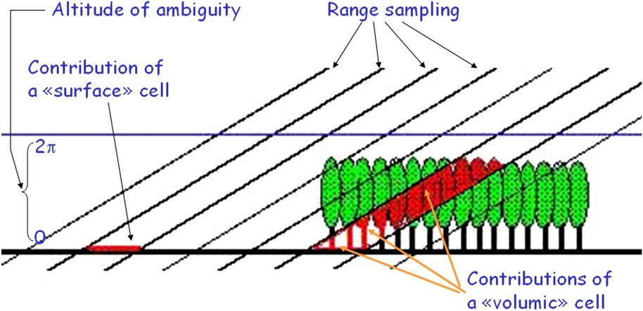
Scheme on volume scattering in case of target penetration by radar waves.
Croquis illustrant la réponse en volume pour les cibles que les ondes radar peuvent pénétrer.
The Shuttle Radar Topography Mission led to an almost global and very homogeneous mapping of the topography of the Earth. Before going into details with this mission, we would like to emphasize the complementary nature of different systems, such as single pass optical systems like HRS. Their contribution to the global topographic map is essential in the following ways: (1) they can deal with uncommon geometric situations where radar is limited, such as deep valleys where shadowing and layover [6] are the rule, (2) they have abilities to operate in urban environment (i.e. with discontinuous elevations) especially with the new development in small baseline stereoscopy, (3) they can lift ambiguities in areas where radar waves (especially in L band) are likely to penetrate the soil. The second point might be alleviated by radar systems with multiple points of view capable of lifting elevation ambiguities such as the cartwheel.
2.4 The SRTM mission
SRTM features a single acquisition by two antennae physically separated. Therefore it eliminates atmospheric and displacement contribution while constraining greatly the ‘orbital error’ because the distance between the antennas is constrained by the supporting beam. The use of the Space Shuttle is advantageous in terms of onboard power. It also provides attitude and orbit control to the C-band radar payload. However, the limited duration of the Shuttle flight led to the use of a wide-swath mode of radar operation, called SCANSAR [3], which reduced image quality. Using this mode also led to a topographic map acquired over a large range of incidence angles. Finally, the beam limited the antenna separation to a non-optimal value of 60 m and its vibration modes made the final processing of the data more difficult.
Nevertheless, SRTM is a turning point in our global knowledge of the planet. The vertical accuracy of 15 m or better on 30-m geographic cells is much more homogeneous than previous global coverage and the public availability of a data is very popular, even at a reduced accuracy and sampling. The resulting accuracy might be considered as limiting for some applications. However, it is very well chosen for a unique dataset. The C-band waves are stopped by the top of vegetation rather than the ground. The difference between the topography of the ground and the topography of the canopy would become significant should the vertical accuracy improve. More generally, such an improvement makes the world's terrain model a renewable resource rather than a single shot. From this point of view, 15-m or so accuracy is optimal.
Another crucial point achieved by the mission is the vertical and planimetric referencing. All the unwrapping has been performed once and for all because any future mission aimed at improving the SRTM terrain model will do it by producing residuals after comparison with SRTM reference. These residuals do not need to be unwrapped as soon as the contour lines produced by the interferometric fringes of the future mission are separated by more than the SRTM error bar. We could almost say the SRTM rendered all kind of unwrapping useless, because rough models are available for topography as well as for most cases of ground deformation. These models can be used to eliminate most of the fringes in an interferogram regardless of their origins, possibly after tuning through a limited set of parameters.
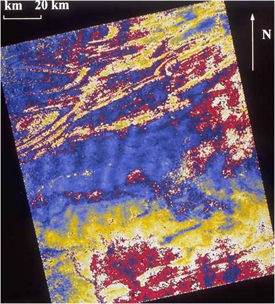
The SRTM mission also embarked a German–Italian dual antenna radar called X-Sar that operated in conventional strip mode. The global coverage could not be achieved by this additional system within the mission duration as shown in Fig. 10, because the images were narrower. On the other hand, the vertical accuracy of this limited dataset is in the order of 5 m.
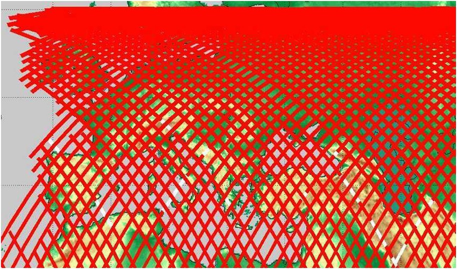
X-Sar coverage over Europe and vicinity.
Couverture de la mission X-Sar au voisinage de l'Europe.
2.5 Future improvements
If we now focus on what is likely to change in the coming years with respect to topographic imaging and radar interferometry [25], the first point is certainly the improvement of civilian radar systems that will feature better resolutions, and in turn relax the interferometric condition and allow much better vertical accuracies. An existing system such as Radarsat I can operate with an altitude of ambiguity of three meters, allowing a sub-metric vertical accuracy. The future X-band systems such as COSMO and TERRASAR, or C-band such as RADARSAT 2 will improve on this, leading to accuracies on the order of 10 cm, but still subject to the influence of the atmosphere in multiple-pass operations. Two interesting possibilities arise with these new systems. The first is to invest on more elaborated processing schemes: for instance, using SRTM as an unbiased terrain model with poor high frequencies due to its limited accuracy and mixing it with the high frequencies generated by the new systems, knowing that the low frequencies of these new datasets are likely to be wrong because of the atmospheric contribution.
Another possibility is to take advantage of several identical spacecrafts and flying them in formation to perform quasi-simultaneous data takes, as it was envisioned for ERS 1 and 2 in 1994 and more recently with RADARSAT 2 and 3, as shown on Fig. 11. There are a few problems raised by such an idea: first, the time difference that ensures a substantially identical atmosphere contribution in both images is not accurately known. For example, if the data takes are separated by 20 s, clouds travelling at 20 m s−1 may cover almost half a kilometre, thus shifting their potential contributions from an image to the next, which therefore will not be fully cancelled in the interferogram. Second, the topographic product features are linked to the stereoscopic baseline, which is likely to vary along the orbit following the laws of orbital mechanics. Third, there is a loss of operational capabilities linked to this mode of operation: having two satellites flying together reduces the overall life span of the system considered as a whole and decreases its revisit capabilities. These systems are the beginning of distributed sensors concepts, which we will detail now.
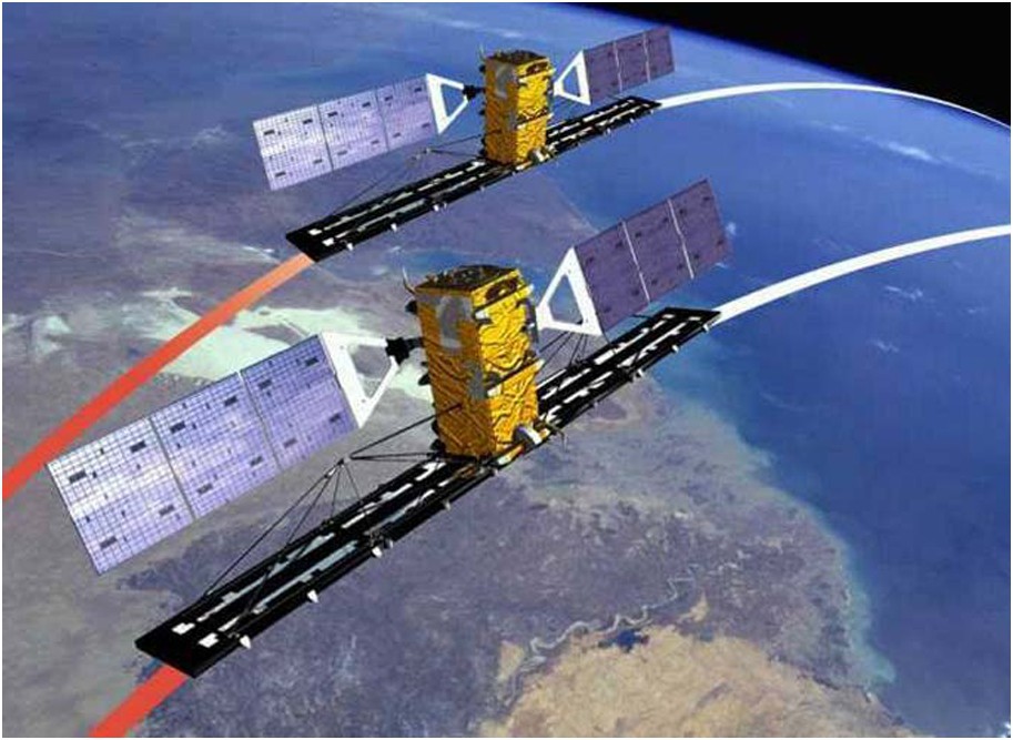
Artist's rendering of Radarsat tandem (from a presentation by P.F. Lee and K. James).
Vue d'artiste du principe de mission en tandem (ici avec Radarsat, d'après une présentation de P.F. Lee et K. James).
2.6 The cartwheel concept
There are many concepts of distributed radar sensors. However, we will illustrate one of them: the interferometric cartwheel system [14].
The system consists on a set of three receivers that listen to the area illuminated by a conventional radar system. Since the power requirement of the receive-only function is very low, we take the opportunity to use microsatellites to implement the concept, which in turns allows us to use three receivers while staying within reasonable cost. The interest of having three receivers is the homogeneity of the topographic product wherever along the orbit, as described later. The drawback is that the receiving antenna onboard each microsatellite is small and gives poor protection against ambiguities in the SAR image [14]. The protection against ambiguities is provided only by the transmitter's antenna. The basic product achievable by the system is a better-than-1-m accuracy up the 80° of latitude on square geographic cells 10 m in size. This result is obtained in six months typically and can be improved by multiple passes and averaging or by tuning the cartwheel configuration to extreme separation after a first model has been acquired.
The main advantage of the system is that it can be added to any radar imaging system for a small fraction of its cost. It does not need to be launched at the same time than its bigger partner or to be jointly designed with it. Fig. 12 displays an artist rendering of the system together with the Japanese satellite ALOS in L band (launched in January 2006). The orbital approach used by the cartwheel is described in Fig. 13. Each microsatellite is placed on an orbit synchronous with the partner's one, but with a slight change of the eccentricity. The change is the same for each microsatellite, but the apogees of the microsatellites are distributed along the orbit. This results in a relative motion of the microsatellites along an ellipse-shaped relative trajectory, with a horizontal axis twice as long as the vertical axis. The relative trajectory is followed by each satellite with the same period as the orbit's one. The advantage is that taking the data of the two satellites best placed for topographic interferometry (that is with the best vertical baseline) gives a very stable result, actually always within 8% of the average value, provided we switch the satellites used as they circle this ellipse to keep only the two optimally spaced. The interferogram of the third satellite might be used of course to improve signal to noise or to lift elevation ambiguity, especially in urban context. This is because this third satellite shows a different separation of the contour lines it produces. The rectangles attached to each microsatellite represent the area of proper interferometric conditions, so these rectangles must intersect if the microsatellites data are to produce interferometry. These rectangles introduce a new dimension of the capabilities of distributed systems.
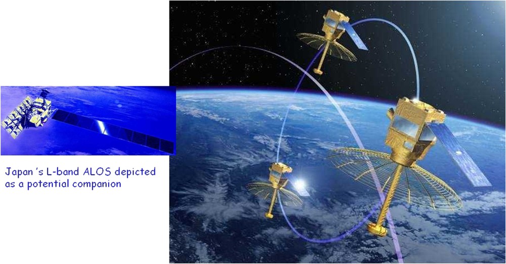
Cartwheel with ALOS (from illustrations by JAXA and P. Carril). The cartwheel constellation may fly 100 km away from its transmitting partner.
Roue interférométrique imaginée en vol avec le satellite ALOS (d'après des illustrations de la JAXA et de P. Carill). La constellation constituée par la roue pourrait voler à 100 km de son partenaire illuminateur.
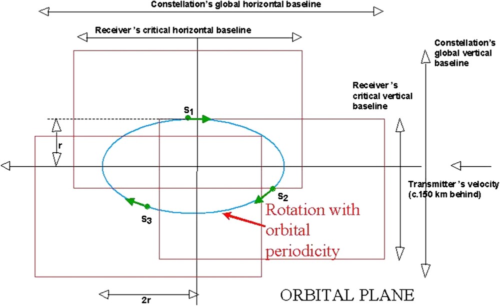
Cartwheel orbital trick. The horizontal and vertical critical baselines indicate the maximum separations allowed vertically (because of the variation of angle of incidence) and horizontally (because of the width of the antenna footprint along the track). These critical baselines would look very similar if expressed in the frequency domain where they would be representing the radar bandwidth (vertical) and the Doppler Effect (horizontal). Such a representation is related to the resolutions of various products: Namely the range resolution (respectively, the azimuth) is inversely proportional to the vertical (respectively, horizontal) frequency span. The resolution of any single image acquired by any of the receivers is inversely proportional, in azimuth and range, to the size of the rectangle attached to these receivers, whereas the resolution of an interferogram computed between S1 and S2 shows a poorer resolution in relation with the smaller intersection rectangle between S1 and S2. On the contrary, a full combination of the three images would yield a better resolution in relation with the union of all the rectangles.
L'astuce orbitale à la base du principe de roue interférométrique. Les bases critiques horizontale et verticale sont les séparations maximales possibles verticalement (à cause de la variation de l'angle d'incidence) et horizontalement (à cause de la largeur de l'empreinte d'antenne le long de la trajectoire). Ces bases critiques ont des significations très similaires si elles sont exprimées en termes d'écarts de fréquences, où elles représentent alors la largeur de bande de l'émission radar (en vertical) et l'effet Doppler (en horizontal). Une telle expression est reliée aux résolutions des images : la résolution en distance (respectivement, le long de la trace) est inversement proportionnelle à la séparation de fréquence verticale (respectivement, horizontale). Donc la résolution d'une image quelconque d'un récepteur (ou d'ailleurs de l'illuminateur) est inversement proportionnelle, en distance comme le long de la trace, à la taille du rectangle attaché à ce récepteur, alors que la résolution de l'interférogramme, calculé, par exemple, entre S1 et S2, sera plus médiocre, en relation avec la taille plus petite du rectangle intersection de S1 et S2. Au contraire, une combinaison complète des trois images donnerait une résolution en relation avec l'union de tous les rectangles, donc meilleure que celle du satellite illuminateur !
The geometry of Fig. 13 can also be understood in the frequency domain: the vertical side of the rectangle then represents the radar bandwidth, as seen by the ground targets, with a vertical offset due to the angle of incidence. The horizontal side of the rectangle corresponds to the Doppler bandwidth, as seen by the ground targets with an offset due to the position of the receiver's antenna. All these frequency bands are inversely proportional to the achievable resolution. As a consequence, the resolution of the images of each individual receiver is the same as the one of the transmitter. The planimetric resolution of the interferometric products between two receivers is poorer because the rectangular intersection of their two rectangles is smaller than the rectangle of a single microsatellite. On the other hand, considering the full frequency span available from the three receivers results in a much larger polygon, if not strictly rectangular, leading to ‘super-resolution’ products [18] after a proper processing has merged all the data. With three microsatellites, the improvement is at most less than a factor of two in both azimuth and range. The concept has been demonstrated using simulation. After an in-flight demonstration, it could be extended to a factor greater than two, using more microsatellites constituting concentric ‘wheels’ of various radii.
The cartwheel mission can achieve a much more accurate topographic map than the SRTM one, and slightly more global in terms of latitude, despite a poor initial image quality due to the small antenna of the microsatellite. This performance is mainly due to the fact that the antenna separation will be much higher. The system is also less complicated in terms of error management, because the laws of orbital mechanics are much smoother than the behaviour of masts in space. As an example, the oscillation of the tip of a mast may act directly on the range to the targets, whereas oscillations of a small spacecraft about its centre of gravity generally do not change the range at first order. The Cartwheel products are expected to benefit fully from the fact that the world topography has already been unwrapped thanks to the Shuttle mission. The cartwheel is an improvement mission and a possible way to renew periodically a global Digital Terrain Model. It may also be a test bed for more advanced spaceborne radar architecture and formation flying.
Pushing the concept further may involve placing a large number of microsatellites ‘paving the frequency plan’ in the manner of Fig. 13, while using several settings of the additional eccentricity. In this more advanced and mature scheme, the transmitter may not be a receiver anymore, which might make it cheaper because low power is never mixed with high power.
The current baseline cartwheel mission is a strawman resulting from an optimal tuning of engineering parameters such as to satisfy a wide spectrum of needs. The typical figures are a vertical accuracy of 70 cm with 10–12-m-wide geographic cells obtained on a global scale, possibly excluding a few degrees of latitude in Antarctica. That is on the part of the planet which is accessed by a typical sun-synchronous radar satellite partner. But the cartwheel product can be tuned in many aspects.
First, once the first coverage has been obtained (in about seven months), another set could be acquired with the goal of bringing down the accuracy to 50 cm in places not dependent on season or producing a seasonal dataset elsewhere (i.e. deciduous forests, ice and snow-covered areas).
Second, after a second pass or instead of a second pass, the cartwheel radius could be extended to the point where the altitude of ambiguity is below the accuracy of SRTM dataset (relying on the first cartwheel dataset to avoid ambiguity removal in a staged approach). Priority could be given to flat areas not active in terms of vegetation.
Third, specific data takes could be acquired such as very low angle of incidence data on stream and water bodies (for continental hydrology), or on rapidly changing topography such as volcanoes deforming with gradients beyond the capabilities of differential interferometry. In some cases, the rate of erosion could be assessed as the measurement is robust with time (in this scheme, the final topomaps are compared, not the radar images used to build them).
Finally, ‘application oriented’ averaging could be performed on the topographic maps. As a significant example, surfaces of water can be observed by interferometry provided the data takes are quasi-simultaneous. Since the high-resolution radar image in amplitude allows the identification of the shoreline of water bodies, a global averaging could be performed on these areas, knowing they share the same elevation in order to exchange a useless planimetric resolution with the best elevation resolution. Averaging over a kilometre-scale water body would better the performance by one hundred in elevation. Unfortunately, this does not mean a vertical accuracy of 7 mm since the water surface is much less bright than the average target unless the angle of incidence is very low. A proper combination of averaging and low incidence angle could nevertheless lead to interesting performances in hydrology for the assessment of continental waters.
3 Conclusion
Topography is a critical measurement for almost all Earth sciences and applications: geologic mapping, hazard assessment, large construction projects, etc. In addition, differentiated topography resulting from surface motion is critical in understanding tectonic and volcanic activities and their resulting hazards. The SRTM data is being widely used, and was recently described as the most dramatic advance in cartography since Mercator.
In this paper we described the concept of radar interferometry and gave an illustrative example of a cartwheel concept that could enable significant advances in our ability of global topographic mapping in the future. This concept utilizes low-cost small satellites that can be flown in formation with traditional synthetic aperture radar systems, thus providing an interferometric network to conduct very high-resolution topographic mapping.
The quest for a more and more accurate description of the global topography will soon underline its time dependence, turning its measurement into a continuous task.