

1 Introduction
The ability of clay soils to act as semipermeable membranes that inhibit the passage of electrolytes may be of great value. Clays exhibit membrane properties when charged ionic species are excluded from the pores, while uncharged species have a relatively free movement. Clays are therefore capable of inducing coupled transport such as osmosis, electro-osmosis, electrodialysis, and thermodiffusion.
The major purpose of this work was to experimentally determine the coefficients that characterize these couplings in compact clays. More precisely, let us consider a porous medium filled by an electrolyte solution with a concentration n (defined as the number of molecules per m3). When a pressure gradient ∇P, an electric field E, a concentration gradient ∇n, and a temperature gradient ∇T are simultaneously applied to the porous medium, four fluxes are generated, namely a flow characterized by the seepage velocity U (m s−1), a current density I (A m−2), a solute flux
| (1a) |
| (1b) |
| (1c) |
| (1d) |
A literature search shows that measurements of these coefficients for clays (and especially for compact clays) were not frequently performed. Interesting contributions concerning electrokinetic coefficients are from Elrick et al. [5], Gronevelt et al. [6] and Sherwood and Craster [19]. To the best of our knowledge, only Thornton and Seyfried [20], and Lerman [10] have contributed to thermodiffusion. A recent review of all of these coefficients was made by Horseman et al. [7].
This paper is organized as follows. Section 2 is devoted to the theoretical determination of the coupling coefficients. The local transport equations corresponding to the electrical potential, the ionic concentrations, and the velocities are solutions of the Poisson–Boltzmann, the convection diffusion and the Stokes equations; these equations are numerically solved and integrated to obtain the macroscopic fluxes. Numerical results for various porous media correspond to the analytical solutions valid for circular Poiseuille flows when the capillary radius is replaced by a suitable length scale.
The material, the experimental procedure and the data are described in Section 3. Two samples of argilite extracted from a Callovo-Oxfordian formation were characterized. Permeability, conductivity, electro-osmotic coefficient, effective diffusion coefficient, osmotic coefficient, coefficient related to “membrane potential” and Soret coefficient measurements are described. Results are considered as functions of solute concentration, porosity and temperature in non-isothermal conditions. Data relative to the electrokinetic coefficients are compared to numerical and analytical results derived by [2] and [12].
2 General
The coefficients
| (2) |
Then, u and the pressure
| (3) |
Finally,
| (4) |
To be solved, the set of Eqs. (2) to (4) is subject to the following boundary conditions on the solid/fluid interface S:
| (5) |
These equations were linearized around equilibrium, made dimensionless, and solved by [9] (and the references therein) for homogeneous porous media that could be represented as spatially periodic media. The coefficients
The only cases which can be solved analytically, are the ones of a plane channel or of a circular tube of radius
| (6a) |
| (6b) |
| (6c) |
| (6d) |
| (6e) |
It is important to note that most numerical results obtained for various types of porous media were shown to be very close to the analytical results (6) when the radius of the tube is replaced by the characteristic length
| (7) |
3 Experimental
The phenomenological coefficients
| (8) |
The relationships between the coefficients
| (9) |
3.1 Materials
The material, supplied to us by ANDRA, is a natural compact argilite extracted in eastern France from a Callovo-Oxfordian formation. The wellbore referred to as EST104 was sampled at two different levels. One at 483.6 m (EST104/2364) and the other at 505.15 m (EST104/2487). Both blocks were used to obtain solid cylinders of thickness 3 mm and diameter 12 mm, or powder. A SEM analysis of the argilite powder shows an heterogeneous structure with many aggregates; because of the careful crushing process to obtain powder from the original block, the average grain radius ranges from 1 to 10 μm. The variability of the samples is discussed in this issue by [14].
The solute was sodium chloride supplied by SIGMA (purity 99.5%). The solvent was pure water filtered by an HPCL Maxima unit. The concentration C was ranging between 10−4 and 10−2 mol l−1.
The samples were equilibrated with the solutions for about a month and any additional and undesirable ion that appears during this initial equilibration phase can be eliminated. During the experiments, HPCL chromatography was performed and the concentration of any extra ions such as calcium was found negligible when compared to sodium.
The zeta potential ζ was estimated by measuring the electrophoretic mobility of clay particles in electrolyte solutions. Since the ratio between
| (10) |
Results for ζ in various NaCl solutions are displayed in Fig. 1.
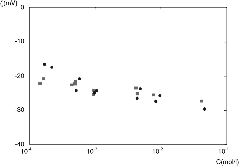
The zeta potential ζ as a function of NaCl concentration C. Data are for: EST104/2364 (■) and EST104/2487 (●). The precision is about 15%.
Potentiel ζ en fonction de la concentration C en NaCl. Les données sont pour : EST104/2364 (■) et EST104/2487 (●). La précision est d'environ 15%.
3.2 Experimental determination of the coefficients K, σ and
3.2.1 Experimental procedure
The experimental cell is detailed in [11] and [13]. The experiments were carried out at atmospheric pressure. The sample, whether it is the original compact rock or the powders, can be compacted or not by means of two porous disks. This compaction limits the swelling that is likely to occur with the addition of sodium chloride. Therefore, various porosities can be obtained for the same sample.
The permeability K was measured by generating a steady flow by means of a constant pressure difference
The sample conductivity σ was measured by a classical method by imposing a constant dc voltage
The electric current was observed to decrease during the measurement time when the electric potential difference is set, probably due to the formation of polarization layers on the electrodes. Simultaneously, a water flow rate
| (11) |
3.2.2 Results and discussion
Results for permeability are displayed in Fig. 2. Note that the permeability obtained for the argilite original sample is in good agreement with the powder permeability.

The permeability K as a function of porosity ε. Data are for: argilite powder (●) and argilite original sample (▵). The precision is about 34% and 24% for small and large porosities, respectively.
Perméabilité K en fonction de la porosité ε. Les données sont pour : la poudre d'argilite (●) et l'échantillon initial (▵). La précision est d'environ 34% et 24% pour les petites et grandes porosités.
In order to study the effects of the compaction pressure and κ, σ was measured for several porosities ε at fixed C, and for several C at fixed ε. It is more convenient to represent the experimental results in terms of the electric formation factor F, which is defined as:
| (12) |
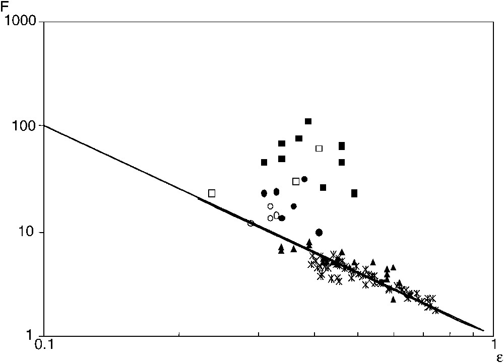
The electric formation factor F (▴) and the diffusive formation factor
The electric formation factor F (▴) and the diffusive formation factor
Facteur de formation électrique F (▴) et facteur de formation diffusif
Facteur de formation électrique F (▴) et facteur de formation diffusif
In Fig. 3, these data are seen to be in very good agreement with the solution of the Laplace equation for various random packings [1]. They can be gathered by an Archie's law,
In Fig. 4, all results are gathered in the dimensionless form
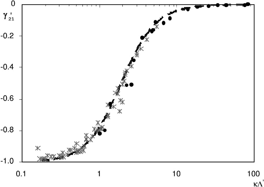
The reduced coupling coefficient
Coefficient de couplage réduit
3.3 Experimental determination of the coefficients
3.3.1 Experimental procedure
The experimental cell was described extensively in Refs. [13,16,17].
Two types of experiments have been performed; the samples were either compacted under different pressures by exerting a compaction pressure during the experiment (EST104/2487) or they were precompacted under a pressure equal to 46 bar before the experiment started (EST104/2364). Thermal regulation with a precision of
The cell was initially assembled with either the less concentrated solution or the more concentrated one and the clay paste was brought to equilibrium with these concentrations. The minimal imbibition time is about 200 h. As a result, the sample was equilibrated with the solution and any additional and undesirable ion that appears during this initial equilibration phase can be eliminated.
Each experiment was divided into two periods. In the first one, a concentration gradient was imposed at a constant temperature of 25 °C. ΔC, ΔP and
The total measured potential difference
| (13) |
Fig. 5 shows typical evolutions of ΔC,
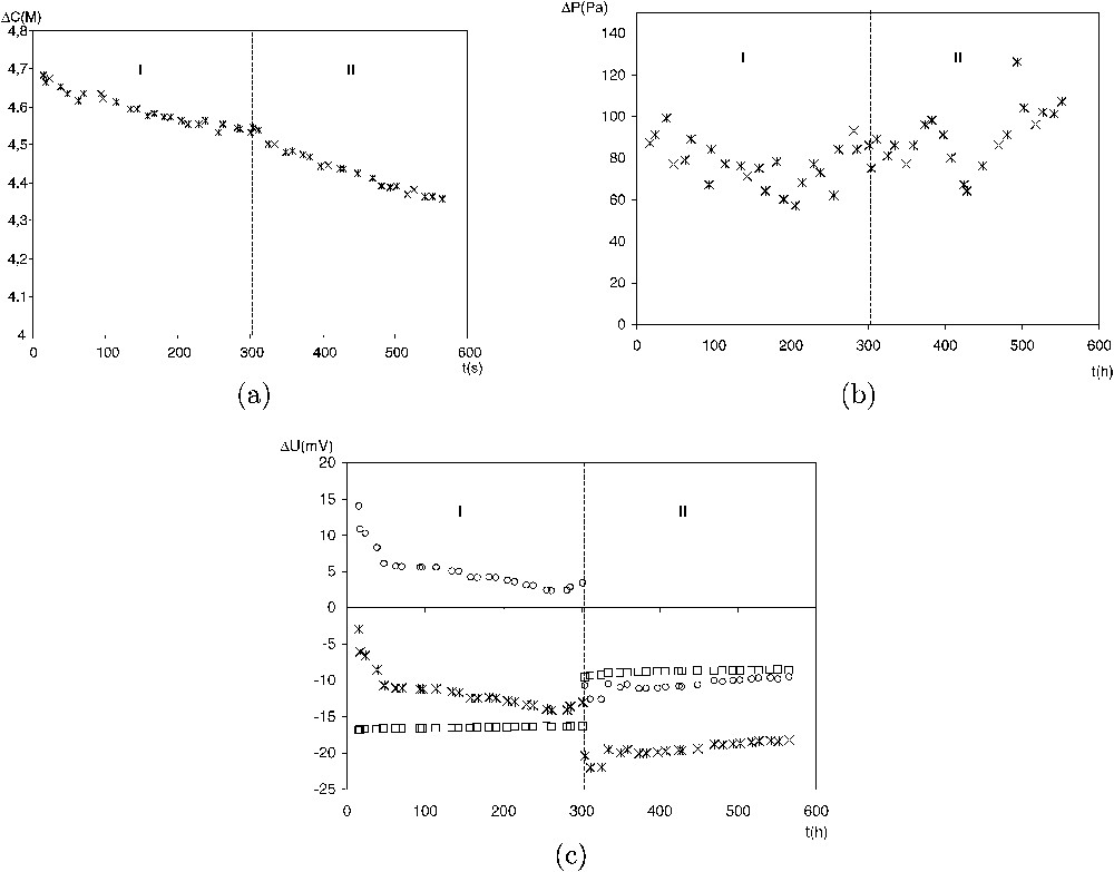
A typical example of the evolution with time of the measured parameters: (a)
A typical example of the evolution with time of the measured parameters: (a)
Exemple typique d'évolution temporelle des paramètres mesurés : (a)
Exemple typique d'évolution temporelle des paramètres mesurés : (a)
The weights
3.3.2 Determination of
During period I, in the absence of any thermal gradient, ΔC, ΔP and ΔΨ decrease with the same rate. Therefore, the ratios
Since the seepage velocity is zero
| (14a) |
| (14b) |
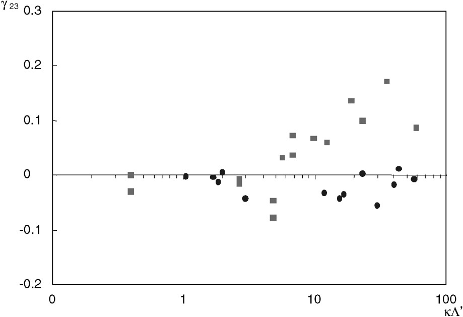
3.3.3 Analysis of
| (15) |
The surface effects on
| (16) |
The coupling coefficient
Coefficient de couplage
The coefficient
| (17) |
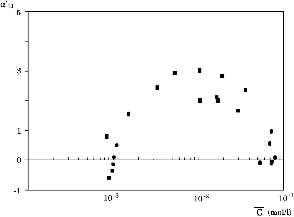
The coupling coefficient
Le coefficient de couplage
The coefficient
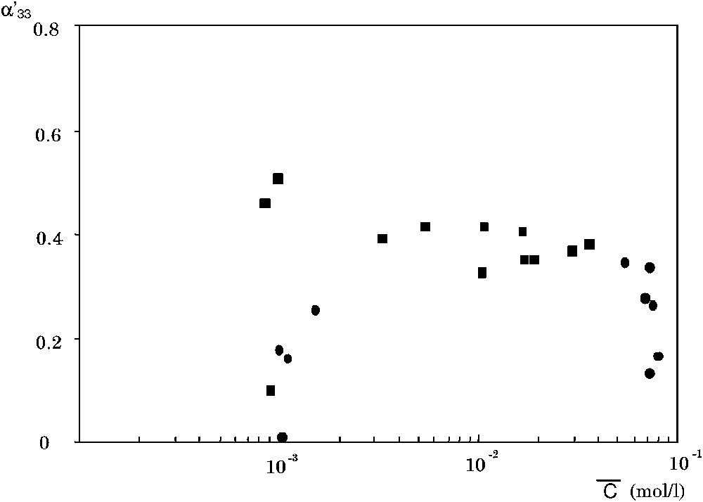
In Fig. 8, we have plotted
The coupling coefficient
Le coefficient de couplage
The hyperfiltration (or inverse osmosis) coefficient
3.3.4 Analysis of the Soret coefficient
Fig. 9 displays the Soret coefficient
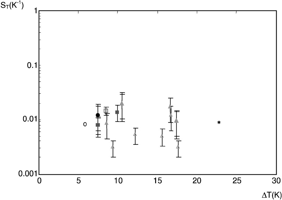
The Soret coefficient
The Soret coefficient
Coefficient de Soret
It is important to note that we have omitted the absolute value in
Let us now compare our results with values obtained in a free medium for sodium chloride [3]. In the free medium,
4 Concluding remarks
The objective of this study was to analyze the behaviour of a compact clay, namely argillite, submitted to concentration, pressure, potential and temperature gradients and to compare the data to theoretical analysis, whenever possible. The coefficients were measured as functions of C and ε. Permeability ranges between 10−18 and
The osmotic coefficient
The coupling coefficient
Non isothermal experiments show that solute transfer is enhanced by thermal diffusion. The Soret coefficients range between
Vous devez vous connecter pour continuer.
S'authentifier