

1 Introduction: First sea-level measurements
Though detailed instructions on how to observe the sea level can be found as early as 1675 in an Italian Journal – an extract appeared in the Journal des Sçavans of 22 April 1675 [53] – the first continuous sea-level observations were published by the geodesists and astronomers Jean Picard (1620–1682) and Philippe de la Hire (1640–1718) in 1680, according to Cartwright [14]. They observed the high and low waters at Brest, France, over a short period of ten days in 1679 [57]. The experience was repeated in 1692 over a five-month period. It proved to be conclusive and led the ‘Académie royale des sciences’ to start continuous observations of the tides at the major French ports. These observations were carried out with the support of the Navy by the ‘professeurs d'hydrographie’, who were asked to measure the sea level according to concise rules established by Goüye and La Hire [27]. Thus, continuous sea level observations have a relatively long history starting in the late 17th or early 18th century. Some sites are still observing today, covering a period of several centuries. Brest is one of them along with Amsterdam, which starts in 1682, Liverpool, in 1768, or Stockholm, in 1774, for instance.
The first devices used to observe the sea level were simple graduated rods, usually called ‘tide poles’, fixed at locations where the instantaneous water-level height of the sea could be read off at any time by an observer. Most of such measurements were restricted to observations of high and low water levels, as well as the time of their occurrences. Their relationship with present-day records is, however, not as straightforward as one could imagine. Important issues on data quality and datum connections need to be addressed before deriving any trend in sea level components. But the exercise of data ‘archaeology’ proves to be valuable today in the context of climate changes due to global warming (e.g., [70]). Automatic recording devices appeared only in the first half of the 19th century: in 1831, in the United Kingdom, at Sheerness; in 1842, in France, at Toulon. These were mechanical gauges, equipped with a float, wires, counterweights, a timepiece, a pen, a paper-chart recorder and a stilling well [73]. They provided the first complete tidal curves that could be examined in detail and digitized for further analysis. These devices stimulated a new enthusiasm for sea-level observations and tidal analysis. For instance, in France, we recently discovered that long sea-level records turn out to be more numerous than the two well-known Brest and Marseilles ones [75].
Tide gauges based on mechanical float devices have lasted for more than 150 years. Still in 1983, a survey conducted by the Intergovernmental Oceanographic Commission (IOC) of the UNESCO showed that 94% of the tide gauges were mechanical [33]. The situation has considerably changed since then. Sea level can be measured either ‘in situ’ at the coast or on the seafloor off-shore, or from space with radar altimetry satellites. The floating gauges have been progressively replaced by new technologies. Modern types of gauges are mainly based either on the measurement of the subsurface pressure, or on the measurement of the time of flight of a pulse, acoustic or radar. The IOC manuals on sea-level observation and interpretation provide valuable detailed information on each type of gauge, their respective advantages, drawbacks, performances and limitations, as well as advice on operational methods and environmental conditions of use [34]. It is interesting to note that the volume I of the IOC manuals includes a test designed by a geodesist named Charles van de Casteele (1903–1977) to determine the accuracy of a tide gauge, proving that geodesists did not restrict their contributions to the early measurements of the 17th or 18th centuries. Moreover, Charles Lallemand (1857–1938), head of the levelling commission in France, designed a gauge called ‘médimarémètre’ aimed at measuring the mean sea level directly [39].
It is worth outlining here that, whatever the technique is employed, the basic quantity provided by tide gauges is an instantaneous height difference between the level of the sea surface and the level of a fixed point on the adjacent land. Thence, tide-gauge records not only include signals stemming from the ocean tide, but also from a large variety of sea-level signals that can be caused by variations in atmospheric pressure, density, currents, continental ice melt... as well as vertical motions of the land upon which the measurement instrument is located. Records of such devices are indicative of relative sea-level changes, whose characteristic timescales range from several minutes to centuries and can be inferred depending on the length of the time series. Many other scientific applications than the natural tidal research and modelling might therefore benefit from tide gauge records. The next sections will focus on three of these applications, in which the local and relative characteristics of the sea-level heights measured by coastal tide gauges will be extensively discussed.
2 Vertical datums
Sea-level data from tide staffs or tide gauges have been used for more than a century to establish vertical reference systems on land and on sea in order to define the height and depth datums. The origin of both types of datum is reviewed in this section: the origin of their definition, what their practical realisations and limitations are, and how space geodesy can solve the problem of their unification.
2.1 Height systems on land
The main elements that define a height-system definition are an origin, a vertical reference surface of zero level, and a type of height, for instance, dynamic heights [30]. The problem of the origin of the national height systems was discussed in the mid-19th century. The question of whether a mean sea level would be more convenient than a low tide level was raised in France in 1847 when the first attempt to define the zero level for all French land levelling was undertaken by Paul-Adrien Bourdalouë (1798–1868) [9]. Finally the concept of geoid was defined as that equipotential surface of the Earth's gravity field that most closely coincides with the mean sea level. The choice of that particular surface was motivated at that time by the belief that the average level of the sea was constant over long periods of time. Consequently most national levelling networks set up their origin using the ‘mean sea level’. Tide gauges were installed along the coasts for that particular purpose. In 1864, the International Association of Geodesy (IAG) further urged maritime countries to carry out continuous sea-level observations at as many sites as possible, and to link them by precise levelling. The foreseen purpose was to provide the future means by which the zero level for all European levelling networks could be established [40].
In practice, the countries usually chose one tide gauge station to compute this ‘mean sea level’ over a certain arbitrary time period. For instance, in France, the current datum was determined at Marseille from continuous tide gauge records performed during the period 1885–1896; in Britain, the Ordnance Datum was determined at Newlyn from records extending from 1915 to 1921. More details can be found in Ihde et al. [32] on the origin of the height systems in European countries. However, whatever the choice of site, the mean sea level varies from place to place and at one specific place over time. Today, the mean sea level at Marseilles is about 11 cm above the local 1885–1897 datum, whereas it is about 20 cm above the Ordnance Datum at Newlyn. Thus, the datums no longer represent the ‘real’ average of the sea level at these sites. Moreover, the mean sea level can differ from an equipotential surface by as much as several decimetres due to steric effects (caused by temperature and salinity) or currents. The deviation of the actual ocean surface from an equipotential surface is known as the ‘sea-surface topography’ and varies spatially. Thus, different gauges, even located along the same coast line, may result in different height datum values.
To summarise, the mean sea level is not an equipotential surface, different height datums may refer to different equipotential surfaces, resulting in constant offsets between them. Space geodesy provides the means to evaluate these offsets in a well-defined geocentric reference system, the International Terrestrial Reference System, or ITRS, for instance [8]. Willis et al. [68] demonstrated the role of tide gauges that are linked to such a frame in the connection of the two French and English levelling datums through the Channel by using the Global Positioning System (GPS). Rapp [58] further established a rigorous procedure that estimates the separation between reference surfaces defined by several vertical datums, and the geoid that is defined by geoid undulations computed from a geopotential model or a gravitational field model. The author applied his procedure to the case studies of England, Germany, Australia and US vertical datums, and confirmed that differences between height systems may reach values of 1 or 2 m. The role of tide gauges that are linked to a geocentric reference system for a global unification of vertical reference systems on land was however demonstrated. Projects like the European Vertical Network (EUVN) have emerged since then with the objective of unifying the different national height datums within a few centimetres based on an integrated network approach using GPS, levelling and tide gauge observations (see for instance [32]). A major outcome has been, however, the resolution of the British sea slope anomaly in the 1990s. A large-scale systematic error in the realisation of the zero-level levelling surfaces was revealed from the tide gauge benchmark connection by GPS. This systematic error led to an ‘apparent’ north–south sea slope when connecting the tide gauges to the national levelling networks (see for instance [2] or [72] for a review). What is the situation of the vertical reference systems at sea?
2.2 Nautical chart datums
Tide-gauge data are also used to establish the datums to which the depths are referred on nautical charts and above which tide predictions are provided for practical purposes. Since 1996, the International Hydrographic Organization (IHO) recommends that the Lowest Astronomical Tide be adopted as the International Chart Datum. This datum is defined as the lowest tide level that can be predicted in average meteorological conditions and in any combination of astronomical conditions. It is a theoretical level below which sea level falls rarely, useful for marine navigation: the mariner is almost always sure to have more water under his keel than displayed on the nautical chart. However, practical realisations often deviate from the theoretical definition. Discrepancies arise mainly from technical limitations. We should keep in mind that many nautical chart datums were established a long time ago, in some places up to two hundred years ago [4]. A rigorous procedure to recover the Lowest Astronomical Tide is available today, developed by Simon [61]. It requires sea-level values, either coming from tide gauges or from hydrodynamic models, harmonic analysis and processing of the tidal constituents through an iterative technique. In practice, the implicit level to which the tidal levels refer and, in particular, the Lowest Astronomical Tide, is the mean sea level over the period of observations used in the analysis. Due to the spatial complexity of the tides, of the mean sea-surface topography and the geoid, the Lowest Astronomical Tide is a rather complex surface reference level. At the time of most nautical chart datums implementation, the knowledge and the tools were rather limited. Observations hardly covered more than a monthly period at a given location. Fluctuations of annual mean sea level values are typically of 5–10 cm, while monthly values may vary by about 10–20 cm. Thus, differences between the theoretical definition and the practical implementation of the reference level may be as large as several decimetres. The nautical chart datum actually presents a rather local extension, which is materialised at the coast near the observation sites by a local set of tide-gauge benchmarks. The main difficulty is, however, the transfer of the tidal datum from the reference stations at the coast to the sounding sites (e.g., [60]).
An open issue in hydrography is the unification of the nautical chart datums as well as a better access to the reference level off-shore to reduce the soundings. Here again space geodetic techniques can provide a solution towards a globally consistent nautical chart datum. Wöppelmann et al. [74] describe a method to map the Lowest Astronomical Tide – the IHO recommended reference level – in a well-defined and maintained geocentric terrestrial reference frame. Provided that the Lowest Astronomical Tide is given with respect to the mean sea level, for instance through the iterative approach described in Simon [61], the connection to the geocentric reference frame can then be performed through a mean sea surface computed from satellite altimetry by subtracting both quantities, as stated in the relationship:
Whereas the idea is quite simple, a rigorous implementation of the method requires the availability of sea-level data provided by tide gauges and hydrodynamic modelling to get the harmonic constituents over the area of interest, as well as an accurate mean sea surface. Both quantities should be available at the same locations and referred to the same sea level observation period. In practice, these constraints usually require geographical and time interpolations. A demonstration study was carried out in the French areas of the Atlantic Ocean and the Channel. The first results were presented at the FIG Symposium held in Malta in 2000, and published after the IAG Scientific Assembly held in Cartagena in 2001 [3]. For most areas, they obtained an error budget within the requirements of nautical chart datum realisation of less than the decimetre. The largest errors arise between the coast and about 25 km offshore. They come from the mean sea surface realisation; either CLS-SHOM98 or CLS01 mean sea surfaces were used in our studies [28,29]. A local least squares collocation method is applied to compute these surfaces on a regular grid of 2-min spacing, about 4-km spatial resolution. Altimetric data from TOPEX/Poseidon, ERS1/2 and Geosat satellites were selected in a 200-km radius around each point of the grid. The spatial domain covered is almost global (80°S to 82°N) where altimetric data are available. The CLS01 mean sea surface uses seven years of TOPEX/Poseidon data (1993–1999), whereas the CLS-SHOM98 mean sea surface uses three years (1993–1995). A more detailed technical description of the mean sea surface computations can be found at http://www.cls.fr. The results of this work can be improved and expanded, in particular, with accurate geocentric station positions of tide gauges, to improve the mean sea surface at the coast, as well as the computation of a mean sea surface that takes into account better altimetric corrections and more satellite data. A more accurate mean sea surface is actually expected in 2006; in particular, it will not be deformed at the coast to fit EGM96, as was the previous one CLS01 (F. Lefèvre, P. Schaeffer and G. Larnicol (CLS), personal communication). The ideas developed here provide insight into a globally consistent nautical chart datum realisation, which is highly recommended by the IHO.
3 Land movements and sea level trends
During the past century, sea-level observations have been recorded by tide gauges at many coastal stations around the world. A major source of uncertainty in estimating sea-level variations from these instruments is the accurate knowledge of vertical crustal movements which are embodied in the sea-level measurements. In fact, tide gauges measure sea-level changes as variations in the relative position between a geodetic benchmark attached to the Earth's crust and the sea surface. Vertical land movements need to be removed from the tide gauge records in order to convert the time series of relative sea-level change to absolute sea levels. At global scale, the vertical crustal uplift due to the isostatic readjustment of the Earth's crust and mantle to the last deglaciation, is the only coherent geological contribution to the long-term sea-level change for which a thorough understanding of the physical process has been achieved [47,56]. Isostatic adjustment is the process by which the Earth attains gravitational balance with respect to superimposed forces. If a gravitational instability occurs, the mantle rises or sinks to compensate this instability. Removal of the Glacial Isostatic Adjustment (GIA) effects by means of a single global model (see for instance [41,56]), however, still leaves in the vertical crustal rates different regional and local isostatic components [21,48,62], as well as tectonic effects, which are difficult to model.
At present, vertical crustal motions at tide gauges can be measured to a high accuracy by means of space techniques such as, for example, the Global Positioning System (GPS) and the Doppler Orbitography and Radiopositioning Integrated by Satellite (DORIS) [64]. Continuous GPS, however, has shown to be the technique of use in this particular application due to the ease of use, high precision, and its direct connection to the International Terrestrial Reference System (ITRS) through the products of the International GNSS Service (IGS). On the other hand, by means of simultaneous GPS measurements performed at tide gauges and at fiducial reference stations of the global reference system, tide gauge benchmarks can be tied in a global well-defined reference system [5,12,13,76]. The possibility to refer the tide gauge data to the same high precision global reference system allows the comparison between the different tide gauge datasets to be made. This was not the case until about 15 years ago when tide gauge benchmark coordinates were mostly available in the different national height systems. A large international effort is presently underway, the TIGA-PP (GPS Tide Gauge Benchmark Monitoring – Pilot Project), in which 102 tide gauges are co-located with permanent GPS stations. Moreover, other GPS stations complement this network in order to define a common reference frame [6].
The long-term sea-level trends at tide gauge stations are measured to about 0.3–0.5 mm yr−1 [76], provided that the time series are long enough (20–50 years). The accuracy required by GPS shall be in the same range; tide gauge positions must be monitored at the level of 10-mm absolute position error, so that a long-term trend with a realistic error of 0.3 mm yr−1 can be obtained over 20 years or so [5]. The current accuracy of GNSS products is 3, 3, 6 mm for weekly mean values of the north, east and up coordinates respectively and 2, 2, 3 mm yr−1 for the associated linear velocities (see for instance http://igscb.jpl.nasa.gov/components/prods.html or [1]). This ensures that the required accuracy is obtained over a decadal time period. The height determination using GPS data is a delicate task because of several reasons: among them, the atmospheric refraction in the troposphere and the geometric weaknesses in the height component of the GPS in general, and the complicated interactions of the GPS receiver and antenna hardware imperfections (like antenna phase-centre variations and multipath). Moreover, with the exception of areas with natural or anthropogenic subsidence, active tectonics and strong seismic events, vertical rates are smaller by an order of magnitude as compared to the horizontal crustal motions, i.e. they are in the mm yr−1 range [5].
The northern Adriatic area, in Italy, is a rapidly subsiding basin. Natural subsidence affects the entire Po Plain and decreases from the south, where it exceeds 1 mm yr−1 to the north. At the local scale, subsidence rates of anthropogenic nature in the order of 10 to 20 mm yr−1, mainly due to ground fluids exploitation, are superimposed onto the natural tectonic component. We present, as an example, the Marina di Ravenna and Venice Punta della Salute tide-gauge stations located in the northern Adriatic, for which long time series of sea-level data as well as continuous GPS records are available. By looking at these centennial time series (Fig. 1), one can notice that the Marina di Ravenna record is characterized by several interruptions. Moreover, the historical information indicates that the tide gauge was moved at least three times before the last instrument change, which took place in mid 1998. The information regarding the tide gauge benchmark levelling is also rather sparse and doubtful. Anthropogenically driven subsidence rates are present in both data series as well as true sea-level variations. With this information available, it is not an easy task to attempt to separate vertical land motions and true sea-level changes. The trends in Fig. 1 provide an indication of the average linear variation observed by means of the tide gauge data over a period of 105 years.
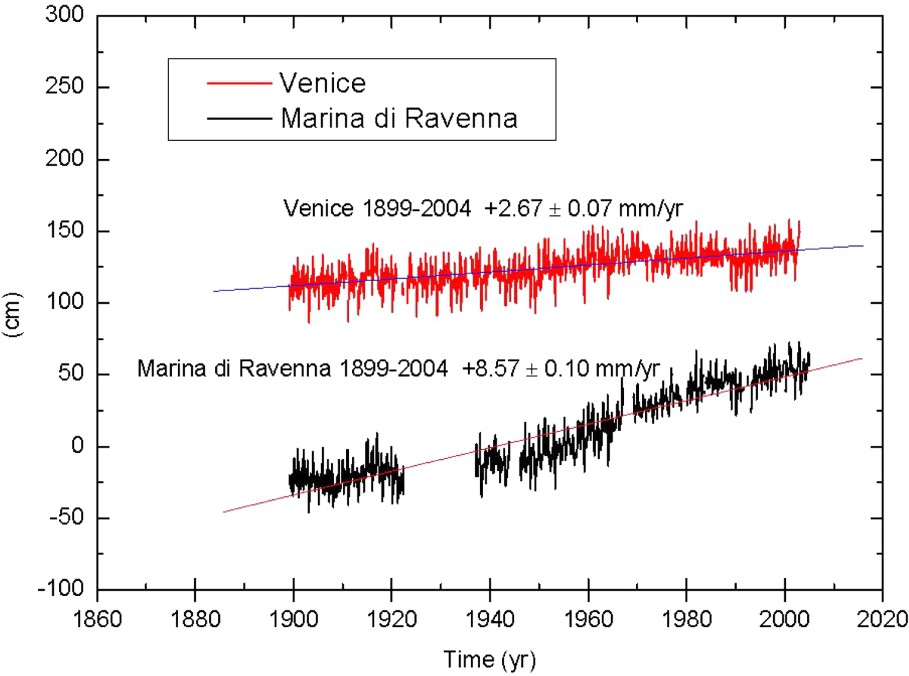
Tide-gauge data series (monthly means) and linear trends for the Venice (top curve) and Marina di Ravenna (bottom curve) stations.
Séries temporelles marégraphiques (moyennes mensuelles) et tendances linéaires pour les stations de Venise (courbe du haut) et de Marina di Ravenna (courbe du bas).
In Venice, anthropogenic subsidence started around 1930 [49,54] and reached a peak around 1970, with different rates during this period of time. Levelling data collected in 1908 and, again in 1961, indicate that there has been a height decrease in the order of 10–15 cm over a period of 53 years, while repeated levelling from 1961 to 1971 indicates an average change of 3 to 4 cm in eight years [10]. After 1970, when ground water control policies were adopted, only a minor subsidence rate is observed [7,11]. Fig. 2 presents the high-precision levelling measurements available for the tide-gauge benchmark and a best-fitting curve providing long-period information on the vertical land motions at Punta della Salute. By removing this curve from the tide-gauge data series shown in Fig. 1, one can derive the local long-period sea-level trend which turns out to be . It can be pointed out that this rate is in agreement with the most recent estimates of global long-term sea rise [51], although it is well known that locally sea-level trends may differ significantly from the global mean.
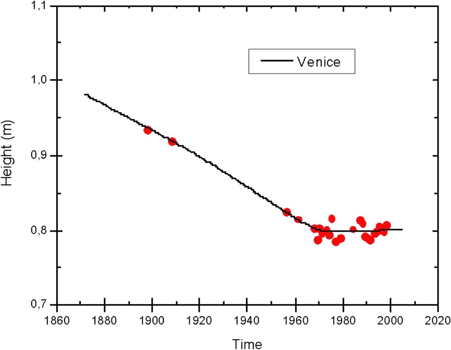
High-precision levelling measurements performed at the tide gauge benchmark at Punta della Salute, Venice.
Mesures de nivellement de précision réalisées sur le repère de marée de Punta della Salute, Venise.
Concerning the last decade or so, it is possible to take advantage of continuous GPS observations at tide gauges. At present, there are two permanent GPS stations located near the tide gauge at Punta della Salute. The one in close proximity (about 10 m) to the tide gauge belongs to the Italian national ‘Servizio Idrografico e Mareografico’. It was installed at the end of May 2005; therefore the available data are not yet long enough for the estimate of a reliable linear trend. The other station belongs to the Italian Space Agency and it is also part of the European Permanent Network (EPN). It is located at a distance of about 1 km from the tide gauge and it can be used, for the time being, to infer the present-day vertical crustal movements. We are aware, however, that it is recommended by international bodies to measure the land movements within 500 m from the tide gauge. Fig. 3 shows, for this latter GPS station, the weekly height time series for the period 2002–2005, created by Kenyeres [38], and the estimated linear trend.
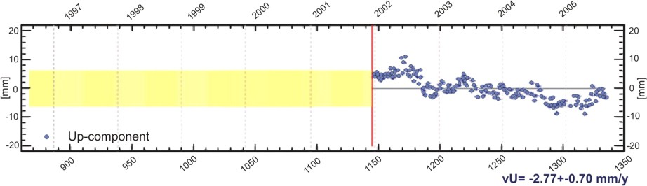
Vertical rate of the Venice EPN station (created by Kenyeres http://www.epncb.oma.be).
Vitesse verticale de la station EPN de Venise (produite par Kenyeres http://www.epncb.oma.be).
The linear tide gauge trend estimated over the 1990–2004 period is . Removal of the land motion as provided by GPS [38] over the past 3.5 years () provides a short-period estimate equal to .
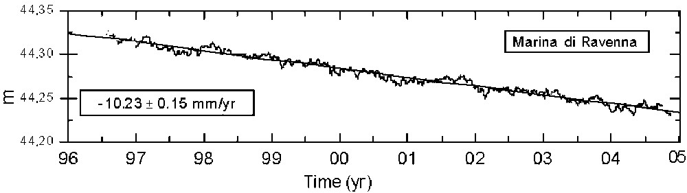
Salvioni [59] reported that, during 60 years from 1897 till 1957, the Adriatic coast of the Emilia-Romagna region subsided by about 20–35 cm, in particular, in the city of Ravenna, subsidence turned out to be 32.2 cm. Gottardo [26] indicated that during the period 1926–1960 in Marina di Ravenna, where the tide gauge is located, there was an average subsidence rate of 7.74 mm yr−1. Starting from 1950, because of intensive ground fluid exploitation, subsidence increased significantly, exceeding 10 mm yr−1. Unfortunately, the levelling data of the tide gauge benchmark referring to the first half of last century are quite doubtful, therefore we attempt to estimate the long-term sea-level trend starting in 1937 after the tide gauge was moved to a new site. Fig. 4 shows the levelling data available.
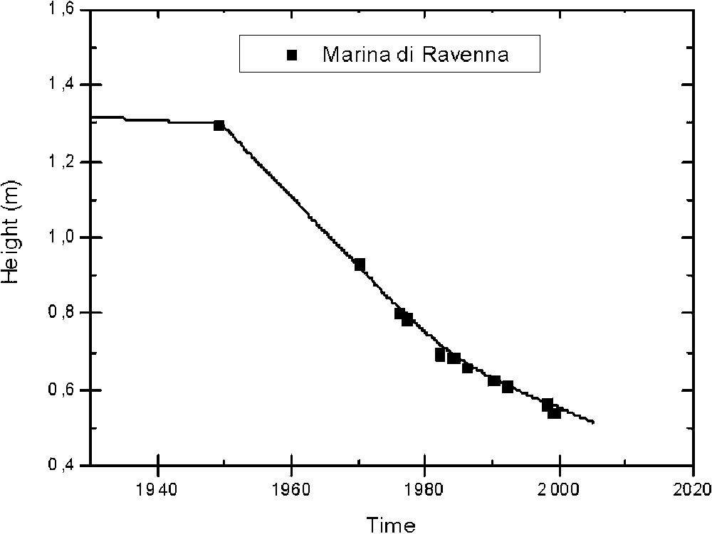
High-precision levelling measurements performed at a benchmark close to the tide gauge at Marina di Ravenna.
Mesures de nivellement de précision réalisées sur un repère proche du marégraphe de Marina di Ravenna.
Removal of the land vertical motion from the tide gauge data series provides a long-term sea-level rise estimate (1937–2004) equal to , in good agreement with the long-term estimate in Venice. Since mid-1996, a permanent GPS belonging to the network of the University of Bologna is operational in close proximity to the tide gauge. Fig. 5 shows the GPS time series of daily height solutions and the estimated linear trend. The trend has been computed after removing a modelled seasonal oscillation [77,78]. The subsidence rate in Marina di Ravenna is still quite relevant and it is confirmed by InSAR data analysis [79].
GPS time series of daily height solutions from which a seasonal model has been removed. Estimate of the linear trend.
Série temporelle des solutions GPS journalières en hauteur, de laquelle un modèle saisonnier a été retiré. Estimation de la tendance linéaire.
The tide gauge linear trend estimated over the period 1990–2004, comparable to that of GPS, turns out to be . Removal of the land vertical movement provided by GPS, , gives an estimate of the short-period local sea-level variation equal to . This rate does not match the one obtained for Venice. There are, at the moment, two possible sources for this difference: (a) the length of the available GPS time series is different: in Venice, there are only 3.5 years of data, while at Marina di Ravenna the series is 8.5 years long; (b) in mid-1998, the tide gauge at Marina di Ravenna was substituted by a new electronic system and no overlap was allowed between the old and the new system.
The two examples shown in this section demonstrate the importance of acquiring in a continuous way high-accuracy tide gauge and vertical motion data at the stations. The lack of this information is the source of relevant discrepancies, particularly in the estimate of the short-period sea-level variations. Comparisons with satellite altimetry data in the northern Adriatic are not easy to perform because the satellite data are limited due to the narrow shape of the Adriatic basin. The next section will however illustrate such an exercise of comparison in the Gulf of Biscay.
4 Sea-level changes at the coast
4.1 Tide gauges versus satellite altimetry
Sea level changes at the coast have traditionally been measured by means of tide gauges. However, the last two decades have witnessed major technological advances in space-borne radar altimetry that have given new insights into the sea level changes of the world oceans. Satellite altimetry provides sea-level measurements relative to a well-defined geocentric reference frame with a wide spatial resolution and a low temporal sampling rate, in contrast to the high temporal and low spatial resolution of the tide gauges. The tide gauges are usually operated with a time sampling of several minutes, whereas altimeter observations are constraint by the repeat period of the satellite, usually between 10–35 days. Therefore, tide gauges are able to describe high-frequency variations, such as seiches or tsunamis, storm surges and any extreme sea-level event, as well as other processes with longer periods, such as tidal waves or secular trends in sea level over the 20th century, whenever long records are available (see previous section). Altimeter measurements seem to be more convenient to determine global mean sea-level change than tide gauges due to the non-uniform spatial coverage of the latter. Global mean sea-level variations have indeed been investigated in previous works, although confident values could not be obtained before the launch of the TOPEX/Poseidon (T/P) satellite in 1992, see for instance [15,17,18,50]. Likewise, satellite altimetry can successfully monitor low-frequency processes of annual and interannual variability. Much work has been carried out on these time-scales in different regions, e.g. [18,23–25,67,71].
One of the main problems of the satellite sea level observations is the aliasing of short-period signals that cannot be resolved due to the coarse temporal sampling of the satellites [55]. The most important contribution originates from tides, which generally account for a large part of the total variance of the sea-level variability. The usual way to correct these effects is the application of a tidal model to remove the most dominant signals. However, these global ocean tidal models do not manage to detect the effects of extreme tidal levels occurring at coastal zones, enhanced by shallow waters. This is true even for the latest versions of high-resolution models CSR3.0 [22] or FES2004 [43]. This imperfect tide modelling may be an important source of error in sea-level determination from altimetry. Altimeter measurements close to the coast are moreover affected by other effects, which degrade the accuracy of the observations: for example, changes of environmental conditions from land to sea unaccounted for in the corrections and corruption of the measurement as soon as the satellite footprint partially covers the land.
Although sampling characteristics and measurement techniques differ, both altimetry and tide-gauge datasets are complementary. Many efforts have been devoted to investigate the relationship between their observations and to determine the origin of the differences, explained in terms of either physical processes or numerical problems. The first comparisons performed were aimed at the calibration of on-fly altimeter observations. The exercise proved worthwhile and allowed the detection of major instrumental drifts for the TOPEX altimeter [45,46]. Sea-level difference time series between ‘in situ’ and space-borne measurements have also been used to infer the vertical crustal land motion at the coast, reaching accuracies up to 1 mm yr−1 at some sites [16,52]. Besides the land movements that may affect the tide-gauge stability, the origin of the differences in sea-level trends computed using both datasets has been widely discussed. For the last decade, altimeter data show lower rates of sea-level rise than tide gauges. Holgate and Woodworth [31] have attributed these differences to an enhanced coastal sea level rise compared to the global averaged sea-level rise.
4.2 Comparison between space-borne and ‘in situ’ measurements
The question that often arises about tide gauges is to which extent they are representative of the open ocean variability. This question can in turn be reverted: to which extent can satellite altimetry observe coastal processes? The high number of studies focusing on such issues seems to indicate that there is not a unique response [16,20,31,36,52,66,69]. It depends upon many factors, like the location of the tide-gauge site and the specific environmental conditions of the surrounding area. A comparison of simultaneous sea-level observations in the Bay of Biscay using T/P and tide gauge data from three sites available in this region (see Fig. 6) will illustrate some of the issues that have still to be addressed. We focus on the period 1993–2001 for which satellite data are available. Sea-surface heights from T/P are computed and re-sampled into fixed along-track bins along the repeated ground tracks of the satellite. These data have been provided by the DGFI (Deutsches Geodätisches Forschungsinstitut) and a manuscript with their description is under work. Sea-surface height data are converted into sea-level anomalies by using the CLS01 mean sea surface model [29]. Usual corrections are applied: dry and wet tropospheric corrections, including the correction for the drift in the wet troposphere [37], ionospheric correction, sea-state bias from the model of Chambers et al. [19], inverted barometer, as well as ocean and loading tidal effects from FES2004 ocean tide model [43].
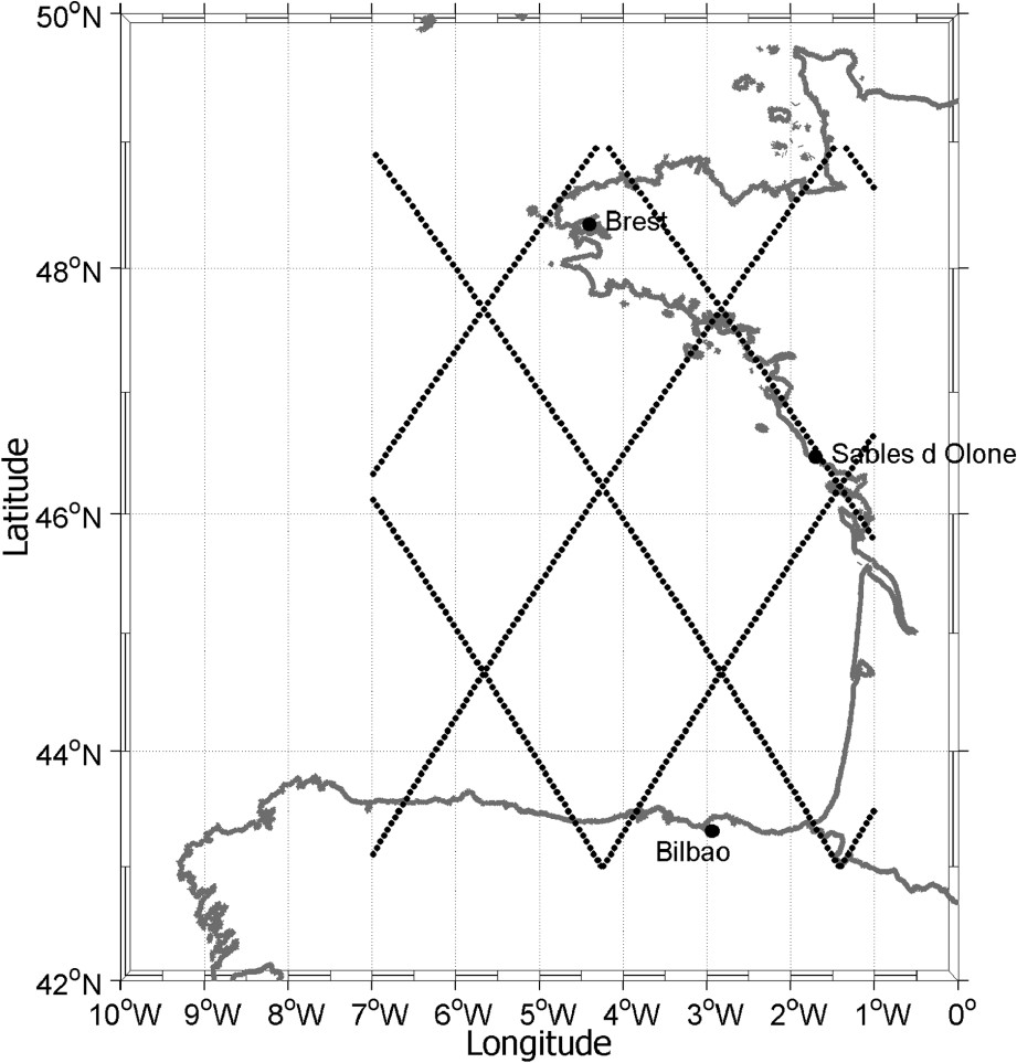
Location of sea level measurements at the Bay of Biscay.
Localisation des mesures de niveau marin dans le golfe de Gascogne.
In order to study the possible differences between sea level at open sea and at the coastal sites, both satellite and tide gauge datasets have to be prepared, so that they can be assumed to measure the same oceanographic signal. This implies that the inverted barometer correction is not applied to the altimeter data, since it is present in the tide gauge observations. Likewise, tidal corrections are not applied. The comparison is performed between each tide-gauge station and the surrounding altimeter observations contained in a radius of 100 km. Sea-level differences are computed between tide-gauge records and sea-level anomalies as measured at the considered bins. The tide-gauge observations are linearly interpolated to the exact time of the satellite pass. Fig. 7 shows the resulting time series and their differences at Brest, Les Sables-d'Olonne and Bilbao.
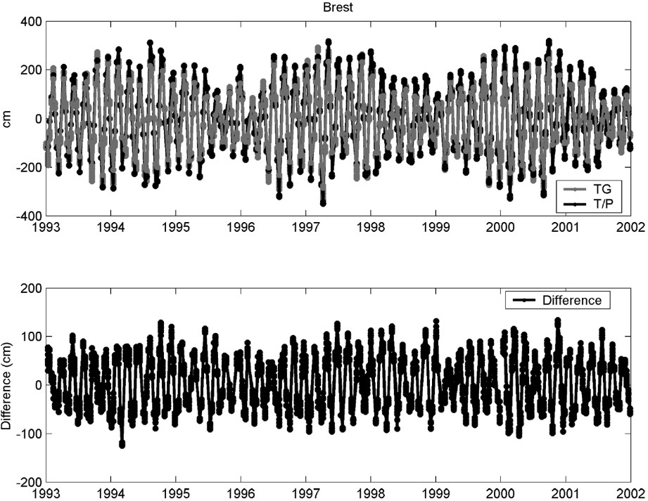
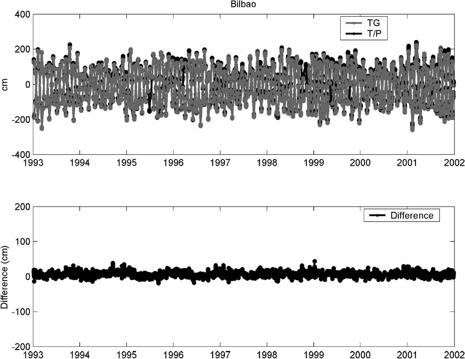
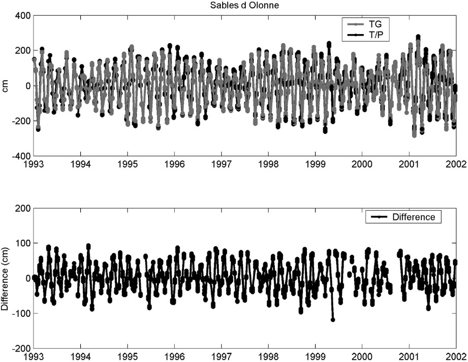
Simultaneous differences between altimetry and tide gauge measurements for stations in Brest, Les Sables-d'Olonne and Bilbao.
Différences instantanées entre mesures altimétriques et marégraphiques aux stations de Brest, Les Sables-d'Olonne et Bilbao.
The main signal that appears in the simultaneous time series (upper panels) is the 62-day aliasing period of the tidal component M2. It is well known that the most important contribution to sea-level variations in the Bay of Biscay is caused by the tides. In particular, the dynamics are dominated by the barotropic semidiurnal tides M2 [42]. Tidal currents are weaker in the southern part of the bay, where the main factors influencing the circulation are storm residuals and density currents. Towards the north, with the growing width of the continental shelf, the importance of the M2 contribution is enhanced. Consequently, it is observed that its amplitude is larger for the northern stations. Moreover, its signature is clear in the difference time series (lower panels), indicating that the M2 amplitude is significantly different at the tide gauge site and at the nearby open ocean. Again, the importance of this contribution is larger at the northernmost stations.
Additional differences were investigated by means of spectral analysis. Besides the dominant tidal signal, there are also annual and semi-annual oscillations in the difference time series. Annual cycle is mainly caused by the steric effect [63], although other effects, such wind or atmospheric pressure, have a small annual contribution too. So it is not surprising that we find a difference in amplitude between the coast and the surrounding area. On the other hand, the semi-annual cycle is mostly a consequence of the atmospheric forcing via inverted barometer effect. In the Bay of Biscay and during the analyzed period, the dominant seasonal signal in atmospheric pressure is clearly semi-annual. It is well known that closed areas do not respond in the same way to the inverted barometer effect, as it is reflected in these records. To summarise, part of these differences can be attributed to different physical mechanisms acting at the coastal zone. The dominant tidal signal in the differences represents the amplification of tidal waves when arriving at shallow waters. Responses to atmospheric pressure variations as well as to the steric forcing are expected to be different too. The remaining differences are still subjected to discussion. The influence of the applied corrections to the altimeter data and their associated errors will be tested in a forthcoming work.
5 Conclusions
To many people, the term ‘tide gauges’ usually suggests the measurement of the ocean tides; however this paper points out that they should rather be called ‘sea-level gauges’, or more specifically ‘relative sea–land-level gauges’. Located on the coast at the interface between sea, atmosphere and land, tide gauges not only record ocean tides, but also a large variety of sea-level signals that can be caused, for instance, by variations in atmospheric pressure, currents or continental ice melt, as well as by vertical motions of the land upon which the measuring instrument is located, due to tectonic changes, isostatic adjustments, volcanism inflation, sediment consolidation, etc. Therefore, tide gauge data have been – and still are – a valuable source of information to a wide range of activities over a large variety of time scales, for scientific research as well as for many practical applications. Past and current issues have been described here, demonstrating the essential role of tide gauges in Geodesy, whereas the synergy with space geodetic techniques has further been emphasised in the related fields of oceanography and sea-level rise due to climate change. The need for a comprehensive sea-level observation system that relies on both altimetry and tide gauges, as well as on space geodetic techniques, such as GPS, and hydrodynamic modelling to link the coast with the offshore, is even more evident when considering events like the Indian Ocean tsunami of 26 December 2004 [44,65]. Tide gauges are definitely at the meeting point of numerous scientific fields. Projects like the Global Sea Level Observation System (GLOSS) are therefore of the utmost importance towards a comprehensive sea-level observation system [35]. This paper has also drawn the attention to the often vague definition of ‘mean sea level’, which subsequently affects the definition of the ‘geoid’ to which is related (see Section 2). When realising these abstract notions, one should specify how the average is computed, which spatial coverage and/or temporal span is considered. Moreover, the sea level being variable over decades, even millenniums, one should attach a reference epoch to each realisation of these quantities, either ‘mean sea level’ or ‘geoid’.
Acknowledgements
Altimetry data have been kindly provided by Wolfgang Bosch of the DGFI (Deutsches Geodätisches Forschungsinstitut) in Munich. The author Marta Marcos acknowledges the postdoctoral fellowships funded by the ‘Conseil général de la Charente-Maritime’ and the ‘Région Poitou-Charentes’. Part of this study has been developed at CLDG (‘Centre littoral de géophysique’) in the framework of the COSSTAGT project, which has been supported by the CNES. Finally, the authors are grateful to Stuart McLellan for his valuable comments.