

1 Introduction
Studies of chemical equilibria involving carbonate solutions often lead to seemingly paradoxical results. Since these studies are essential for the understanding of the ocean-atmosphere system behaviour it may be useful to recall the main, well understood points of these studies, as well as the still pending and unanswered questions. The present article wants to be a synthetic presentation of results and arguments dispersed in the literature for the last 20 years, and present in the comprehensive textbooks [14,31]. In no way has it the ambition to pretend to be the totally original vision, but we think that it can help nonspecialists of geochemistry to better evaluate the state of knowledge of this fundamental system. After a brief recall of chemical equilibria in the carbonate system we shall present a few simple models of the preindustrial ocean which allow to propose a chemical composition of the ocean during a glacial period, then to discuss which possible processes may be at work to change the carbonate system during an interglacial–glacial transition.
Carbon dioxide concentrations of air bubbles trapped into Antarctic ice are positively correlated with temperatures deduced from isotopic composition of hydrogen and oxygen in ice [22,38]: interglacial periods display CO2 concentrations of 280 μatm versus 180–200 μatm for glacial periods.
The Milankovitch theory [33] relates glacial–interglacial alternances to insolation variations and points to the temperature as the primary variable, CO2 concentration variations being the consequence of temperature variations. While some observations [13,49] have suggested that CO2 increase precedes temperature increase, it now seems well established [17] that temperature increase comes first, hence that temperature is the leading variable.
Whatever the preferred initial hypothesis, the explanation of CO2 variations has generated many studies and hypotheses [4,14,25,41–43].
The main goal of this article is a didactical presentation of these hypotheses, favouring simplicity more than precision. It is meant for nonspecialists of ocean geochemistry to understand the major concepts linked to carbon dioxide exchanges between ocean and atmosphere and the inherent difficulties. The main conclusions, rather easily demonstrated by that approach, are in good agreement with results obtained by more precise, but rather “opaque”, calculations [14].
As previously stated, chemical equilibrium in carbonate solutions frequently leads to seemingly paradoxical results. Hence, after recalling the main aspects of these equilibria, we present some simple models of the preindustrial ocean. Then, we shall apply these models to determine the chemical composition of the ocean during a glacial episode. And finally, we discuss which are the main likely processes which make the carbonate system vary when going from a glacial to interglacial period.
2 Chemical equilibria in the carbonate system
2.1 Interactions with the gaseous phase: Henry's law
For a gas G in a gas mixture, the partial pressure p(G), proportional to its volumetric proportion, is linked at equilibrium to its concentration in the aqueous phase, [G], by Henry's law:
| (1) |
The equilibrium is attained within a time which depends mainly on the surface agitation. There may exist a certain difference between pressure p’ in the gas and the pressure p in the aqueous phase calculated according to the above formula. Equilibrium is achieved in about one week but one to two months can be necessary in the case of CO2. As we are usually interested in steady state situations, at the time scale of the century, we can limit ourselves to the calculation of pressure in the aqueous phase and admit that equilibrium between the aqueous and gaseous phases is indeed achieved.
2.2 Acid-base reactions in sea water
CO2 is an acid gas which reacts with water to produce hydrogenocarbonate HCO3−, then carbonate CO32− ions by dissociation
When CO2 is added to a solution it gives a mixture of these three species and this results in an increase of the quantity DIC, whose common name is “total dissolved inorganic carbon”. DIC is defined by:
| (2) |
DIC can be modified only by CO2 additions to the solution or CO2 production in the solution.
The three species also obey two other equations:
2.2.1 Acid-base equilibrium
with the corresponding mass law action:
| (3) |
This equilibrium is instantaneous. Hence Eq. (3) is always verified.
2.2.2 Electroneutrality of the solution
For all natural waters this applies to all main ionic species.
| (4) |
Among these ions only carbonates, hydrogenocarbonates and some minor species (b− in the above equation, among which [H3O+] and [OH−]) are able to fix or liberate H + ions. All other ions are inactive with respect to H+. Regrouping active species on one side and inactive species on the other we obtain:
| (5) |
I call the sum on the right side the “alkaline reserve” (AR) [2,31]. Each of its terms can be modified only by addition or in situ production of inactive species. Like DIC, AR is a conservative quantity obeying simple mixing laws. The left side is alkalinity which can be very accurately measured by means of a titration with strong acid. For all theoretical study, it is easier to predict changes in AR, from which changes in alkalinity are derived.
| (6) |
Eqs. (2), (3) and (6) allow us to calculate [CO2], [HCO3−] and [CO32−].
In sea water the minor species b− is the borate ion, an active base which is not completely negligible:
| (7) |
A precise study should take care of borates, which I have done in numerical calculations (captions of Figs. 2 and 3). For the present simplified description, I neglect borates. Then:
| (8) |
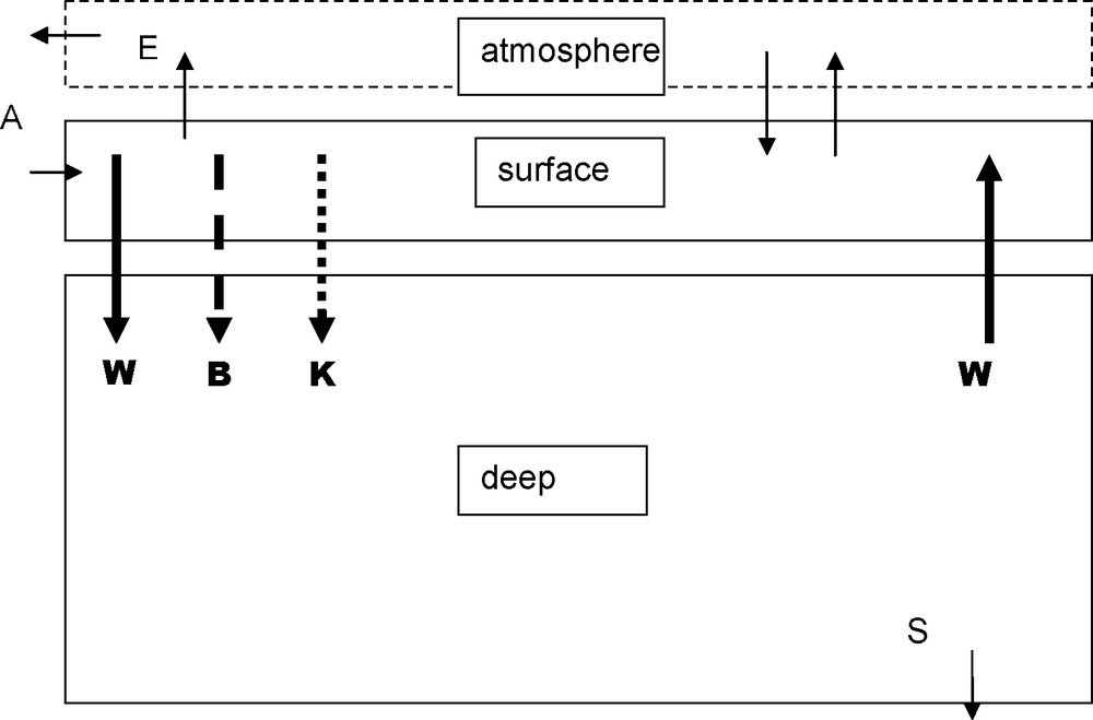
Two boxes model. Data for the main parameters are in the following table: indices s and d refer to superficial and deep boxes. A and S arrows stand for continental weathering and sedimentation; DIC and AR inputs are in the order of 0.01.1015 mol/year. For sedimentation RA∼ 0.01.1015 mol/year and DIC ∼ 0.005.1015 mol/year, the difference (CO2) is released in the atmosphere (E) and weathers the continental limestones.
Modèle en deux boîtes. Les valeurs des paramètres principaux sont regroupées dans le tableau suivant : les indices s et d correspondent aux boîtes superficielle et profonde. Les flèches A et S correspondent à l’altération du continent et à la sédimentation ; les apports de CID et de AR sont de l’ordre de 0,01,1015 moles par an. La sédimentation de AR a la même valeur ; celle de CID 0,005,1015, le reste de CID part dans l’atmosphère (E), puis va altérer le calcaire sur le continent. Masquer
Modèle en deux boîtes. Les valeurs des paramètres principaux sont regroupées dans le tableau suivant : les indices s et d correspondent aux boîtes superficielle et profonde. Les flèches A et S correspondent à l’altération du continent et à ... Lire la suite
| Period | W | B | K | DICS | DICd | RAS | RAd | P(CO2) |
| Pm3/year | Pmol/year | Pmol/year | mol/m3 | mol/m3 | eq/m3 | eq/m3 | μatm | |
| Interglacial | 1 | 0.27 | 0.068 | 1.96 | 2.25 | 2.33 | 2.37 | 290 |
| Glacial | 1 | 0.35 | 0.018 | 2.20 | 2.52 | 2.72 | 2.67 | 199 |
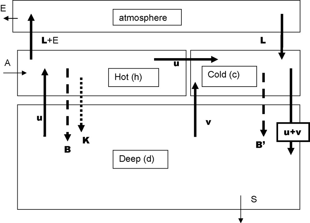
Three boxes model. Data for the main parameters are in the following table: indices h, c and d refer to hot, cold and deep boxes respectively A and S arrows stand for continental weathering and sedimentation; DIC and AR inputs are in the order of 0.01. 1015 mol/year. For sedimentation RA = 0.01.1015 mol/year and DIC ∼ 0.005.1015 mol/year, the difference (CO2) is released in the atmosphere (E) and weathers the continental limestones.
Modèle à trois boîtes. Les indices h, c et d se rapportent respectivement aux boîtes chaude, froide et profonde. Les valeurs des paramètres principaux sont regroupées dans le tableau suivant : les flèches A et S correspondent à l’altération du continent et à la sédimentation ; les apports de CID et de AR sont de l’ordre de 0,01,1015 moles par an. La sédimentation de AR a la même valeur ; celle de CID 0,005,1015, le reste de CID part dans l’atmosphère (E), puis va altérer le calcaire sur le continent. Masquer
Modèle à trois boîtes. Les indices h, c et d se rapportent respectivement aux boîtes chaude, froide et profonde. Les valeurs des paramètres principaux sont regroupées dans le tableau suivant : les flèches A et S correspondent à ... Lire la suite
| Period | u | v/u | B/u | K/B | B′/B | DICh | DICc | RAh | RAc | RAd | RAd | p(CO2)h | p(CO2)C | O2,d |
| Pm3/a | mol/m3 | mol/m3 | mol/m1 | eq/mJ | eq/m3 | cq/m3 | μatm | μatm | mol/m3 | |||||
| Interglacial | 1 | 1.1 | 0.26 | 0.25 | 0.01 | 1.97 | 2.15 | 2.30 | 2.33 | 2.38 | 2.55 | 279 | 279 | 0.16 |
| Glacial | 1 | 0.7 | 0.26 | 0.25 | 0.35 | 1.89 | 2.06 | 2.55 | 2.33 | 2.36 | 2.67 | 190 | 190 | 0.05 |
In seawater, [CO2] is negligible relative to [HCO3−] and [CO32−] in (2).
Thus, (2) (3) and (8) lead to:
| (9) |
| (10) |
| (11) |
| (12) |
The K′B product is a function of temperature: its value is 0.010 atm.(mol/L)−1 at 2 °C and 0.035 at 30 °C for S = 35‰. It also varies with salinity S. For salinities close to average ocean values (35‰), it decreases by 1.5% when S increases by 1 ups.
These four equations have been widely used in Broecker and Peng's book [14]. They allow a very satisfying first approach of the carbonates’ problem in sea water. I shall use that approach for the qualitative description.
2.3 Interactions with the solid phase: calcium carbonates
“Carbonate ions” react with calcium ions to give solid calcium carbonate under two possible forms: calcite and aragonite.
At equilibrium
| (13) |
Equilibrium is reached only after a very long time and the kinetics of these reactions in a complex medium like sea water are still very badly known.
In sea water, Ca2+ concentration is constant. Hence, we only need to compare measured CO32− concentration to equilibrium concentration.
| (14) |
[CO32−] decrease will favour dissolution, [CO32−] increase carbonate precipitation.
3 Processes modifying DIC and AR
Three important processes (and the three corresponding back processes) are able to modify the DIC of sea water:
- • dissolution (outgassing) of gas;
- • respiration or oxidation of living organisms (photosynthesis);
- • dissolution (precipitation) of CaCO3.
Let us examine the effects of each of them on AR.
3.1 Gas dissolution
When we dissolve Δ moles of CO2 per liter of solution, the increase of DIC is Δ and that of AR is zero, because no species intervening in the constitution of the AR are modified. Hence [CO32−] ≈ AR–DIC, decreases, which favours CaCO3 dissolution and not calcite precipitation as some people might think [1].
This also produces an increase of p(CO2), which looks reasonable. What is not so evident is the magnitude of that increase; AR is greater than DIC by around 10%; an increase of DIC by a few percentage means a relative decrease of DIC – AR 10 times larger, and an increase of the numerator in Eq. (11). The relative increase of dp(CO2)/p(CO2) is much larger than dDIC/DIC. The ratio of these quantities, called the Revelle factor, is around 10.
For an exchange of an inactive gas, this ratio would be equal to 1.
CO2 loss by outgassing would evidently lead to opposite results.
3.2 Respiration
By respiration, I mean any oxidation of living matter or matter of living origin. Such a reaction may be schematized by:
That reaction is a source of energy for living organisms.
Average atomic ratios C/P (=1/y) and N/P (=x/y) of oceanic organic matter are known as Redfield ratios [40]. Their respective values are 106 and 16. Then, x = 0.15 and y = 0.01. We shall neglect y.
NO3− is an inactive species entering “AR” with a minus sign. A production of Δ moles of CO2 per liter corresponds to a decrease of x.Δ mol/liter for AR. Decrease of [CO32−] and increase of p(CO2) are larger than in the case of gas dissolution.
The opposite reaction is photosynthesis which produces living matter from CO2, nitrogen and phosphorus with the help of solar light as energy source.
Photosynthesis favours calcite or aragonite precipitation; it is, unequivocally, the main mechanism for both authigenic and biogenic CaCO3 formation in nature.
3.3 Dissolution of CaCO3
CaCO3 dissolution liberates one calcium ion for each carbonate ion. Ca2+ enters AR with a factor 2. Hence AR increases by 2Δ when DIC increase is Δ. CO32− increases and p(CO2) decreases. Inversely, CaCO3 precipitation induces an increase of p(CO2). There again some old high school “souvenirs” (acid attack of a limestone producing CO2) might lead, by wrong intuition, to think the contrary.
3.4 Anaerobic oxidation of organic matter
When oxygen is lacking only a few bacterial species are able to get energy from organic matter oxidation by other inorganic oxidants (nitrates, ferric iron, sulphates…), results are quite different from those obtained with oxygen [31].
Take for example ferric iron. The reaction is:
In that realm, NH4+ and Fe2+behave like inactive species. For Δ moles of CO2, AR increases by (8 + x)Δ and [CO32−] by (7 + x)Δ.
Limestones deposited in anoxic sediments will thus be protected against dissolution while under similar temperature and pressure conditions, they would be dissolved if oxygen was present.
4 Lysocline and carbonate compensation depth
Fig. 1 compares measured carbonate ion concentration with calculated equilibrium concentration in the presence of calcite, as a function of depth. The measured concentration essentially depends on the action of the photosynthesis–respiration couple: photosynthesis is predominant at the surface, making [CO32−] grow. Respiration is the only actor in dark deep zones, and [CO32−] decreases.
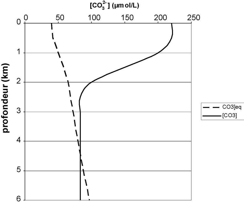
Mean measured carbonate ion concentration (—) and equilibrium concentration with calcite (- - -) versus deptḧ.
Concentration effective en ion carbonate (—) et concentration à l’équilibre avec la calcite (- - -) en fonction de la profondeur.
[CO32−]eq slightly grows with decreasing temperature which corresponds to the observed increase down to 1500 m depth. Below, pressure influence dominates. This curve can hardly change with time, because, at these depths temperature does not vary. The curve is also rather insensitive to salinity variations, the slight increase of K's with S being balanced by [Ca2+] increase.
In surface waters [CO32−] > [CO32−]eq and precipitation is the only possibility.
Around 4000 m depth, the two curves cross each other and dissolution occurs below that depth. Observation of deposits allows one to see a level where dissolution traces are visible. This defines the lysocline [6] which corresponds to calcite saturation. Calcite disappears totally a few hundred meters below the lysocline. The corresponding depth is called the carbonate compensation depth (CCD) [9,11,27]. The CCD corresponds to the depth where dissolution kinetics compensates sedimentation input.
Analysis, in the sediment, of the evolution of CCD or lysocline depth with time is an useful tool for an insight of the carbonate system in the past.
5 Biologic pump and calcareous pump
Oceans and lakes alike, heated from above, have a thermal structure with a lighter and hotter layer above a colder and denser one. That thermal stratification is linked to a chemical one: photosynthesis dominates in the surface layer whereas the deep layer sees only respiration reactions.
The conceptual result of that situation is that ocean is divided into several “boxes”, supposed to remain homogeneous, and between which people try to estimate water, dissolved matter and particulate matter fluxes.
5.1 Two boxes model
Fig. 2 presents the two boxes’ model [21]. The two boxes yearly exchange an amount of water W estimated from carbon-14 studies to be about 1015 m3/year. [1,14]. The amount of inorganic carbon (DIC) exchanged corresponds to:
- • the transport by water;
- • the organic C transfer by gravity from the surface box where it is formed toward the deep box where it is decomposed. This mechanism has been called “biologic pump” (B) or “Williams–Riley pump” (a large part of the organic matter is already decomposed in the surface box);
- • the downward flux of calcium carbonate formed in the surface box (mostly as shells or skeletons) and dissolved in the deep box.
CaCO3 precipitation makes [CO2] increase in the surface box and calcite dissolution causes [CO2] decrease in the deep box. That “calcareous pump” transfers, often not quantitatively, CO2 from depth to surface. Moreover, if temperature or chemical composition of the two boxes are different, the quantities consumed and produced are different also. This confirms that the “pump” notion has to be limited to the conservative quantities AR and DIC. The “calcareous pump” (Calc pump) (K) removes DIC, and twice that amount of AR from the surface box which are transferred to the deep box.
For what concerns the biologic pump (Bio pump), the living organic matter formed in surface by photosynthesis makes DIC decrease and AR slightly increase in that box. The two pumps have opposite roles on [CO32−] ≈ AR−DIC. This is not surprising, because calcite precipitation is a feedback reaction induced by the [CO32−] increase due to photosynthesis.
In the ocean, the biologic pump drives four to five times more carbon than the Calc pump. Hence, the surface box will be relatively enriched into [CO32−] and depleted for p(CO2) with respect to the deep ocean, and that difference will increase with the difference between the efficiency of Bio and Calc pumps.
Since photosynthesis uses preferentially 12C, the surface layer is enriched in 13C with respect to the deep ocean.
| (15) |
The fluxes, expressed in Fig. 2 in 1015 mol/year show that internal transfers are one or two orders of magnitude greater than river inputs and sediment deposits, which thus can be neglected in a first approximation.
The biologic pump efficiency is limited primarily by the level of phosphorus inputs into the surface box, where that element's concentration is very low. If Pp is the phosphorus concentration in the deep ocean and (C/P)MO the Redfield ratio, then:
| (16) |
The system then is almost totally constrained – only K may vary.
On the other hand, that model is unable to explain the dissolved oxygen concentrations: it always predicts a totally anoxic deep ocean.
5.2 Three boxes’ model
Sarmiento and Toggweiler [47], and Siegenthaler and Wenk [48] simultaneously proposed a model with the ocean divided into three boxes plus the atmospheric box, illustrated by Fig. 3. The extra oceanic box, the cold box, corresponds to high latitudes. There is no water going from the hot (surface) box toward the deep ocean box. Vector u corresponds to the “conveyor belt” defined by Broecker and Peng [14] to which is added vector v representing an exchange of water between cold and deep boxes. The “hot” biologic pump exhausts all the available phosphorus, while the “cold” pump uses only a fraction (α) of it. The “calcareous” pump exists only in the hot box. When setting v/u = 1.1 and α at a very low value allows to get parameters’ values close to the average values estimated for the preindustrial ocean with p(CO2) = 280 μatm, [O2]deep = 170 μmol/L and (δ13C)deep−(δ13C)hot = −2.2‰.
6 Trying to reconstruct the ocean's carbonate system during a glacial period
Water from ancient oceans subsists only in sediments’ interstitial water, where it suffered notable changes due to early diagenesis [10]. The reconstitution of the chemical composition of a “fossil” ocean water is very tricky, not to say impossible, problem. Nevertheless, the informations coming from sediments and polar ices corresponding to the last glaciation allow to place certain constraints on variables concerning the carbonate system and to estimate the concentrations corresponding to a steady state.
6.1 Glacial period simulation constraints
The average temperature of surface ocean during glacial age was lower by 2 ± 1 °C than nowadays [5,19,20]. This difference is significantly lower than the difference derived from the Antarctic ices (≈10 °C). Sea level was lower by 120 m [23]; the ocean volume hence was smaller by 3.5% and its salinity higher by 3.5%.
Atmospheric CO2 pressure was 190 μatm [22]. That lowering was equivalent to 0.5% of the ocean's carbon content. That carbon was not stocked in the biosphere. That information stems from the δ13C of glacial carbonate sediments which are lower by 0.4 [4] to 0.7‰ [14] than those of present-day carbonate sediments.
The only reservoir very low in 13C is biosphere (δ13C ≈ −23‰). Part of the carbon of previous interglacial biosphere was in the glacial ocean, representing about 2 to 3% of the carbon dissolved in that ocean. That transfer corresponds to the oxidation of organic matter, which slightly lowers (0.3 to 0.4%) the “AR”. Hence, the 3.5% decrease of the ocean's volume causes a DIC increase of 7% but of 3% only for AR.
From Eq. (12), we see that, relative to the preindustrial situation, “glacial” K’.B is lowered by 20% because of the lower temperature and increased by 1.5% because of the higher salinity; the “chemical composition factor” increases by 60 to 80%. This would lead to a glacial atmospheric CO2 level of 360 to 450 μatm, much larger than the concentration measured in Antarctic ice. The only solution is to imagine a vertical heterogeneity of the ocean with a surface layer richer in [CO32−] and a lower p(CO2).
6.2 Two boxes model
Broecker and Peng [14,15] succeeded in reconstructing the carbonate system of the glacial ocean with two data:
- • the δ13C difference between the surface layer and the deep ocean is not the same during glacial and interglacial periods;
- • the lysocline depth looks rather similar during these two periods.
To this we can add the CO2 pressure in glacial atmosphere.
6.2.1 δ13C between surface and depth
δ13C of pelagic organisms has been compared to that of benthic organisms. The study is difficult because δ13C varies with foraminifera species and called for an elaborated statistical treatment. The results seem to show that the difference (δ13C)surface –(δ13C)deep goes from −2.1‰ during interglacial to −2.7‰ during glacial periods.
From Eq. (15), assuming no change in W, it results that Bio pump was 30% more efficient during glacial periods.
6.2.2 Depth of the lysocline
The discussion of § 4 has shown that the depth of the lysocline constrained the CO32− concentration in the deep ocean.
Archer et al. [4] consider as demonstrated the fact that the lysocline was about the same during glacial and interglacial periods, which sets the CO32− concentration in the deep box to about 80–90 μmol/L in both periods.
6.2.3 Evaluation of the glacial carbonate system characteristics
Starting from the composition (DIC and AR) of the preindustrial deep ocean, and applying the multiplying factors of § 6.1. (i.e. increases of DIC and AR of respectively 7 and 3%), we obtain a first estimate of the glacial deep ocean in AR and DIC. We dissolve enough calcite to bring back [CO32−] to the average value of 85 μmol/L determined in 6.2.2.
The value of the Bio pump efficiency deduced from carbon isotopes leads to a first estimate of AR and DIC in the surface box and Ca CO3 is adjusted so that p(CO2) = 190 μatm, the value trapped in ice bubbles.
At each step an iterative calculation allows to introduce the borate concentration to better represent the situation. In fact, before CaCO3 precipitation, p(CO2) = 197 μatm (Fig. 2) and CaCO3 precipitation will increase that value. Hence, the hypothesis which best corresponds to the observed results is no precipitation at all.
With this simple model we totally constrain the carbonate system of the glacial ocean, but the absence of any CaCO3 precipitation is unlikely.
Broecker and Peng [14] obtained a similar result before calcite precipitation, which they nevertheless envisaged, with a ratio for the Calc and Bio pumps identical to that of the interglacial period. That leads to p(CO2) = 235 μatm.
6.3 Three boxes model
With such a model, and keeping the same AR and DIC values than in the two boxes model, the ways of obtaining p(CO2) = 180 μatm in both hot and cold boxes are increased. We may either decrease calcite precipitation in the hot box, or lower the v/u ratio, or finally increase the biological pump efficiency for the cold box. Available observations are not enough constraining to choose between these three possibilities.
One of the only constraints is not to decrease too much [O2]deep, because the glacial ocean apparently was not anoxic.
The use of more complex models, with more boxes or using general circulation models would be justified if the level of information was sufficient, which is not presently the case for the glacial ocean.
Obviously, these models are very simplistic and, for instance, it has been recently pointed out [28,35] that the coastal zone plays an important role in the ocean C cycle.
7 Processes able to modify the carbonate system during the glacial–interglacial transitions
If the glacial carbonate system reconstructed by the above method is valid, we still need to understand how we move from a “glacial” to “interglacial” state and inversely.
The atmospheric CO2 concentration is controlled at two levels:
- • the surface ocean where the Bio and Calc pumps build a [CO32−] excess and a [CO2] deficit relative to the bulk ocean;
- • the deep ocean where a return of the lysocline to the same depth after each glacial–interglacial (G → I) or the reverse (I → G), keeps [CO32−] to the same value during the two periods.
We still need to identify the processes which allow this brutal change of pumps’ intensity and those which keep the lysocline at a constant depth.
7.1 Modification of the hot box's Bio pump efficiency
δ13C data seem to indicate that the biological pump was more efficient during glacial than interglacial period. Nevertheless, Toggweiler [50] was able to obtain a 13C enrichment of the deep ocean, by solely modifying its ventilation.
The efficiency of the biological pump is linked to the phosphate concentration in the deep box and the Redfield(C/P) ratio (cf. Eq. (15)).
Some authors have imagined an increase of Redfield (C/P or N/P) ratios. This is possible, since a value of (C/P) up to 300 has been observed in some lakes [32], but that hypothesis is strictly unverifiable and shall not be further discussed.
The phosphorus residence time in the ocean is around 100,000 years. Hence, a significant and brutal variation of the deep ocean P can result only from a catastrophic event. This can be the brutal destruction of a major part of the biosphere, as must have occurred at the interglacial–glacial transition (I → G). That destruction has increased the C content of the ocean by 2 to 3%. The P/C ratio being around 10 times larger in living matter than in bottom sea water, this means a 20 to 30% increase of the P amount and of 25 to 35% for its concentration following the ocean shrinkage in volume. That increase is thus sufficient to explain the increase of the Bio pump efficiency for the I → G transition, but this mechanism is not at all adequate for the reverse event G → I.
7.2 Modification of the Calc pump
CaCO3 precipitation results from photosynthesis, which produces a [CO32−] increase. The maximum efficiency of the Calc pump is thus linked to that of the Bio pump.
Archer and Maier-Reimer [3] introduced the expression “rain ratio” when speaking of the ratio C of living matter/CaCO3 and consider this ratio (one may think that the difference rather than ratio would be appropriate) as a key factor for the “glacial CO2” problem. Box models from § 6 however show that the influence of the Calc pump on p(CO2) is relatively minor.
In sea water, the Calc pump proceeds essentially from coccolithophoridaes’ tests and foraminifera shells. It is nowadays about four to five times less efficient than the Bio pump. A priori, the K/B ratio may vary within broad limits. In lakes emplaced in limestone grounds (Léman lake and lac du Bourget) where calcite precipitation is mainly inorganic, Groleau [24] observed a similar efficiency for the two pumps. The minimum K/B value could be zero. However, Ridgwell [43] thinks that calcite may act as a kind of ballast and that if K is too small it can cause a decrease of B. This is possible at the sediment level, which is the main interest of the author, but does not apply to the transfer into the deep ocean box. Indeed, if organisms’ debris do not reach that box they liberate phosphorus in the surface box. That phosphorus will be used by other organisms, and the phosphorus mass balance in the surface box, where its concentration is close to zero, imposes that the amount exported downwards always compensates the amount brought upwards by deep waters upwelling (cf. Eq. (16)).
7.2.1 The silica hypothesis
It supposes that the phosphate arriving in the surface layer is consumed by siliceous (diatoms) rather than calcareous organisms. With sufficient silica inputs the development of siliceous organisms would prevent the growth of calcareous organisms. The present ocean is for the most part of it not rich enough in silica to allow this mechanism to take place.
Tréguer and Pondaven [51] propose that silica inputs by dust, much more abundant during the glacial period, would have allowed siliceous organisms development at the expense of calcareous organisms. That hypothesis is partly supported by negative correlations between calcite and opale, the maximum opale concentrations corresponding to glacial periods.
7.2.2 The corals
Sea water level was lower by 120 meters during the glacial period [23]. This lowers the surface of neritic zones, where corals are deposited, by a factor around 4 [34]. Indeed coral deposits are much more abundant during interglacial than glacial periods [26,34]. This is not exactly a Calc pump modification, but it produces similar effects: a strong coral production corresponds a high p(CO2), a weak production to a low p(CO2). That coral reefs hypothesis [8] is one of the most interesting, but its effect on p(CO2) seems to be not large enough [44].
7.3 Modification of the efficiency of the cold box's Bio pump
The low productivity of cold oceans and particularly the austral ocean is attested by the high phosphate concentrations in their surface waters. Martin [30] supposed that, in these zones, the limiting factor was not phosphate but iron. Indeed ferrous iron enrichment experiments have spectacularly increased the productivity [12]. The accumulation rates of iron in Antarctic ices are 10 times larger during the glacial period [37], linked to a larger rate of deposit of atmospheric dust [39]. The three boxes’ model shows that an increased efficiency of the cold Bio pump was very efficient to make p(CO2) decrease. However, using general ocean circulation models, Maier-Reimer et al., [29] and Archer et al., [4] showed that this effect was not large enough.
7.4 Stabilization of the lysocline depth
This result is still controversial. On one hand, observations by Catubig et al. [18] show that the lysocline depth stays about constant during glacial and interglacial periods. Accordingly, the CO32− concentration should remain constant as well. In the second hand, paleo pH measurements, using boron isotopes [45,46] indicate that pH was about 0.3 units higher during the glacial period in the deep Pacific Ocean. Such an increase means that [CO32−] would in fact be twice larger, implying that calcite could not dissolve anymore. I think that this is questionable and I consider with Archer et al. [4] as a well established fact the stability of the lysocline depth.
The lysocline return to a stable depth can be explained by “carbonate compensation” [4,52]. Any disequilibrium between altered CaCO3 inputs from continents, which can also be modified by an increase in weathering during glacial periods [36] and outputs by burying into sediments give rise to changes in the ocean carbonate system until fluxes’ equality is restored. For example, an increased efficiency of the biological pump gives way to a decrease of [CO32−] and to a rising of the lysocline: as a response carbonate dissolution makes [CO32−] increase.
Hence, we should observe dissolution processes at I → G transitions and precipitation processes at G → I transitions. In fact, Broecker and Sanyal [16] did observe dissolution episodes at the outset of glaciations and Berger [7] described an episodic lowering of up to 3 km of the lysocline depth for aragonite in pteropods at the beginning of the last interglacial episode.
8 Conclusions
Several hypotheses have been brought forward to try to explain how the CO2 atmospheric concentration can be decreased by 90 μatm when going from an interglacial to a glacial period:
- • an increase in the efficiency of the biological pump caused either by an increase of the ocean phosphate concentration or by modifications of the Redfield ratios;
- • an increase of cold oceans’ productivity by eolian input of iron;
- • a decrease of CaCO3 precipitation in surface ocean due to a competition between calcareous organisms and diatoms, or to a reduction in volume of the neritic zones.
None of these modifications or combination of these modifications is able to explain the observed variations of p(CO2). On top of that, the time constants of these processes are seldom compatible with observations.
The different models of calculation used to associate these various changes do not take into account the same phenomena as leading factors. Summarizing we may conclude like Archer et al. [4]: “We conclude that in spite of the importance of understanding the natural carbon cycle, the solution of the mystery of the glacial/interglacial CO2 cycles still eludes us”.
Acknowledgements
My thanks go to Marc Javoy who not only encouraged me to write this article but also carried out the translation. His comments, as well as those of Marc Benedetti, Alexis Groleau and Bernard Sanjuan have indeed improved its quality.