

Version française abrégée
Les données météorologiques, qui ne remontent qu’à quelques siècles au plus, ne permettent pas d’explorer la gamme complète de la variabilité du climat de la Terre. À l’inverse, les données géologiques et, en particulier, les enregistrements fournis par les sédiments marins et les glaces polaires ont montré qu’au cours du Quaternaire, une succession de périodes glaciaires avait été entrecoupée par des interglaciaires de plus courte durée [2,15]. Ces variations périodiques ont été expliquées par la théorie astronomique des paléoclimats [16], mais on commence à peine à comprendre les grandes rétroactions internes au système climatique qui permettent d’amplifier le signal d’insolation pour entraîner une perturbation majeure du climat. Nous nous limiterons ici à présenter une brève synthèse de la variabilité des interglaciaires du dernier million d’années, documentés à la fois par les sédiments marins et les glaces polaires.
Trois aspects essentiels sont apparus (Fig. 1) :
- • l’amplitude des variations glaciaires/interglaciaires du niveau de la mer (et donc des variations du volume des calottes glaciaires présentes sur les continents) a été plus importante dans la période 0–430 000 ans BP que dans la période précédente (430 000–900 000 ans BP), où le niveau des mers est toujours resté en dessous de −20 m par rapport au niveau actuel pendant les interglaciaires ;
- • les températures de l’air en Antarctique présentent également des valeurs plus faibles qu’aujourd’hui pendant les interglaciaires antérieurs à 430 000 ans BP ;
- • depuis 430 000 ans BP, les teneurs en CO2 de l’air ont oscillé entre approximativement 180 ppm pendant les périodes glaciaires et approximativement 280–300 ppm pendant les interglaciaires, alors que ces teneurs ne dépassaient jamais 260 ppm, pendant la période 430 000–800 000 ans BP, couverte par le forage antarctique au Dôme C [25,36]. L’ensemble de ces données suggère donc une relation étroite entre le climat et le cycle du carbone.

Evolution of the climate system over the last 800,000 years. From top to bottom: (i) atmospheric CO2 concentration [36]; (ii) air temperature at Dôme C [19]; (iii) sea level derived from benthic foraminifer δ18O [23]; (iv) 21 June insolation at 65°N [4].
Évolution du système climatique au cours des 800 000 dernières années. De haut en bas : (i) concentration en CO2atmosphérique[36] ; (ii) températures au Dôme C [19] ; (iii) niveau de la mer déduit du δ18O des foraminifères benthiques [23] ; (iv) insolation le 21 juin à 65°N [4].
Caillon et al. [6] ont montré que, lors de la transition glaciaire/interglaciaire datant de 240 000 ans BP, l’augmentation des teneurs en CO2 avait débuté 800 ± 200 ans, après le début du réchauffement en Antarctique, mais avait précédé de plusieurs millénaires la fonte des calottes glaciaires de l’Hémisphère Nord. Par ailleurs, le refroidissement des pôles lors de l’entrée en glaciation précède la baisse du CO2 [29]. Ces résultats confirment que ce n’est pas le CO2, mais les variations d’insolation qui initient la déglaciation [24] et, qu’en revanche, l’augmentation des teneurs en CO2 agit comme une rétroaction amplifiant le réchauffement et permettant la fonte des glaciers de l’Hémisphère Nord.
Ce mécanisme peut être illustré par une série de simulations de la dernière déglaciation, réalisées avec le modèle de climat de complexité intermédiaire CLIMBER, couplé à deux modèles tridimensionnels et thermomécaniques d’évolution des calottes polaires pour l’Hémisphère Nord et l’Antarctique [8,31]. Dans sa version standard, le modèle est forcé par les variations d’insolation [4] et de CO2 atmosphérique [29]. Pour tester l’impact relatif de ces deux forçages sur le processus de déglaciation des calottes glaciaires de l’Hémisphère Nord, des expériences supplémentaires ont été réalisées en maintenant l’insolation ou le CO2 à leur niveau glaciaire. L’évolution du volume de glace de la calotte nord-américaine, simulé dans chacune de ces expériences (Fig. 2), montre le rôle prépondérant de l’insolation pour la fonte de la calotte canadienne, les variations du CO2 venant simplement amplifier le réchauffement et accélérer le processus de déglaciation.

Simulated ice volume of the Laurentide ice sheet for the four sensitivity experiments carried out with the coupled CLIMBER-GREMLINS-GRISLI model: (i) the model is forced by the variations of both insolation and atmospheric CO2 (black solid line); (ii) CO2 is fixed to 190 ppm throughout the simulation with variable insolation (grey dashed line); (iii) insolation is fixed to its LGM value throughout the simulation with variable CO2 (grey solid line); (iv) both insolation and atmospheric CO2 are fixed to their LGM values (black dashed line).
Simulation du volume de la calotte glaciaire Laurentide pour quatre expériences de sensibilité, menées avec le modèle couplé CLIMBER–GREMLINS–GRISLI : (i) le modèle est forcé par les variations de l’insolation et du CO2atmosphérique (courbe continue noire) ; (ii) le CO2est fixé à 190 ppm, avec insolation variable (courbe tiretée grise) ; (iii) l’insolation est fixée à sa valeur du maximum glaciaire avec CO2variable (courbe continue grise) ; (iv) insolation et CO2atmosphérique sont maintenus à leur valeur glaciaire (courbe tiretée noire).
La dernière période interglaciaire, datant de 129 000 à 118 000 ans BP, présente des caractéristiques notoirement différentes de l’Holocène (les derniers 10 000 ans). Le niveau de la mer était supérieur à celui de l’actuel de 4 à 6 m [17]. Les températures de l’air, supérieures de 2 à 5 °C à celles d’aujourd’hui dans le domaine arctique [7,27] sont suffisantes pour expliquer une fonte partielle du Groenland [11] qui ne rend compte que d’une montée du niveau de la mer de 3 m tout au plus.
Il faut donc envisager une fonte partielle des glaces antarctiques. Le réchauffement de l’air au sud de 40°S ne dépassait guère 2 °C [22,37,38], ce qui est insuffisant pour provoquer la fonte de la glace sur le continent Antarctique. Cependant, on peut remarquer que la calotte Antarctique de l’Ouest est peu stable. En effet, contrairement à l’Antarctique de l’Est et au Groenland, une importante partie de cette calotte ne repose pas sur un socle rocheux, mais flotte au-dessus des mers australes. Ces plates-formes de glace jouent un rôle d’arc-boutant pour l’écoulement provenant de la partie de la calotte posée sur le socle rocheux. Elles sont épaisses de plusieurs centaines de mètres et ancrées sur quelques îlots rocheux. Leur base est baignée par l’eau circumpolaire Antarctique, dont la température vers 600 m de profondeur est maintenue voisine de +2 °C par la remontée de l’eau profonde Nord-Atlantique (NADW), qui est plus chaude que l’eau de fond formée sur le plateau continental Antarctique. L’épaisseur des plates-formes de glace de l’Antarctique de l’Ouest et la calotte elle-même sont très sensibles à la température de l’eau circumpolaire avec laquelle leur base est en contact [32].
En mesurant la composition isotopique des foraminifères benthiques ayant vécu pendant la dernière période interglaciaire, Duplessy et al. [14] ont montré que la NADW avait été plus chaude (0,4 ± 0,2 °C) et plus salée (0,04 ‰) qu’aujourd’hui. À l’aide d’un modèle du système couplé océan–atmosphère, ces auteurs ont montré que le réchauffement de la NADW était la conséquence de la forte insolation des hautes latitudes de l’Hémisphère Nord, là où les eaux superficielles plongent à grande profondeur pendant l’hiver (Fig. 3). Le modèle, dont la simulation présente un bon accord avec les données géologiques, montre également que le réchauffement de la NADW s’était transmis aux eaux circumpolaires qui étaient plus chaudes qu’aujourd’hui de 0,3 ± 0,2 °C. Un tel réchauffement peut sembler modeste, mais il a des conséquences importantes : les données satellitaires obtenues par interférométrie radar ont montré que le taux de fonte à la base de la banquise augmente et que le point d’ancrage de cette banquise recule de 10 m par an, lorsque la température de l’eau circumpolaire qui lèche la banquise augmente de 1 °C [32].
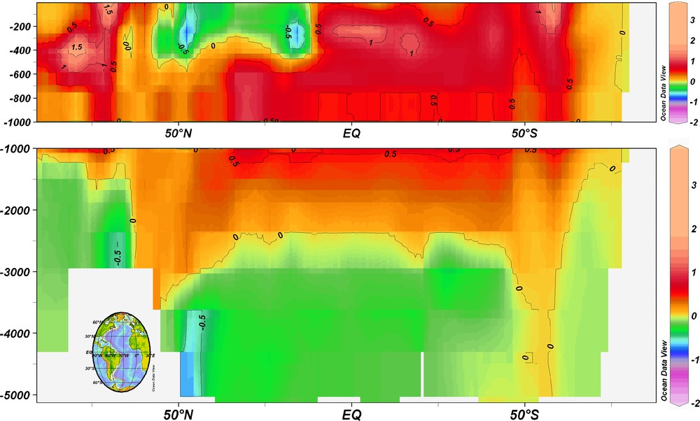
Annual mean temperature anomalies (LIG − modern) simulated by LOVECLIM (in degree°C) along the western boundary of the Atlantic Ocean. The field is averaged over the last 100 years of the simulation. The inset map shows the path chosen for the section.
Différence des températures moyennes annuelles des eaux du bassin ouest de l’océan Atlantique (LIG − moderne), simulée par le modèle LOVECLIM (en degré Celsius). La carte montre la position de la section.
Les données géologiques mettent donc en évidence une gigantesque téléconnexion à longue distance : un réchauffement des hautes latitudes de la zone Nord-Atlantique est susceptible d’entraîner une fonte significative de la calotte de l’Antarctique de l’Ouest et une remontée de plusieurs mètres du niveau de la mer. Les données océanographiques ont montré que les eaux circumpolaires se sont réchauffées de 0,2 °C dans la seconde moitié du xxe siècle [18]. C’est la moitié de celui de la dernière période interglaciaire. Si cette tendance devait se maintenir, l’évolution de la calotte glaciaire Antarctique de l’Ouest pourrait devenir une composante clé des variations du niveau de la mer dans le futur.
Ce sont également les variations de l’insolation, dont les effets sont amplifiés par des rétroactions internes au système climatique qui provoquent la fin d’une période interglaciaire. Les données géologiques témoignent d’un refroidissement d’environ 2 °C au milieu de la dernière période interglaciaire, il y a environ 120 000 ans [10,35]. Celui-ci a été associé à une baisse de salinité des mers Nordiques et une remontée de NADW [9]. Cette perturbation a conduit à un changement majeur de la circulation océanique profonde il y a 115 000 ans [1].
En forçant le modèle couplé océan–atmosphère IPSL-CM2 avec les paramètres de l’insolation d’il y a 115 000 ans, Khodri et al. [21] ont montré que le refroidissement des hautes latitudes qui en résultait a entraîné une augmentation du transfert de vapeur d’eau vers les hautes latitudes, davantage de précipitations, une baisse des salinités et une convection hivernale moins intense dans les mers de Norvège et du Groenland, ainsi qu’un ralentissement de la circulation thermohaline. Le modèle simule également la présence de neige pérenne au Nord du Canada et de la Scandinavie, là où les calottes glaciaires ont commencé leur développement. Dans cette expérience, le taux d’accumulation des neiges est insuffisant pour fabriquer les calottes glaciaires au rythme de 1,6 millions de kilomètres cubes par an (estimé d’après les analyses isotopiques des sédiments marins), mais la rétroaction de la végétation n’a pas été prise en compte. Or le remplacement de la forêt boréale par une toundra augmente beaucoup l’albédo continental et favorise le développement de la glaciation [12].
En conclusion, les données géologiques et des expériences simples effectuées à l’aide de modèles climatiques confirment que la teneur atmosphérique en CO2 et la circulation océanique constituent deux rétroactions majeures amplifiant les variations d’insolation qui initient les oscillations glaciaires/interglaciaires. Les diverses périodes interglaciaires du dernier million d’années ont eu des caractéristiques différentes et l’étude du dernier interglaciaire montre qu’il suffit de faibles variations de la température de l’air dans la zone Nord-Atlantique pour provoquer la fonte partielle à la fois du Groenland et de la calotte glaciaire Antarctique de l’Ouest, en raison d’une téléconnexion à longue distance due au transport de chaleur par la NADW. La calotte glaciaire Antarctique de l’Ouest, située aux hautes latitudes de l’Hémisphère Sud, réagit donc à un signal d’insolation sur l’Hémisphère Nord, transporté par la circulation océanique profonde.
1 Introduction
Meteorological records are too short to capture the full range of climate system variability, which is documented by geological data. 18O analyses of deep-sea cores showed that there were numerous ice ages separated by shorter interglacial periods. Many theories have tried to explain their occurrence, but changes in the Earth’s orbital parameters, which lead primarily to changes in the intensity of the seasonal cycle of solar radiation, are now thought as the fundamental driver of glacial/interglacial oscillations [16]. Increasing the tilt of the Earth’s axis increases the amplitude of the cycle: winters are colder and summers are hotter in both Hemispheres, since the summer Hemisphere intercepts more solar radiation. The temporal variation of the tilt has a period of approximately 41,000 years. The effect of precession on insolation is less straightforward, but together with the rotation of the ellipse around the sun, it determines the time of the perihelion, i.e. the point of the Earth’s orbit which is closest to the Sun during the year. The variation of the time of perihelion has a period of approximately 21,000 years. The perihelion is now reached in January, so that the northern Hemisphere winter is slightly milder and the southern Hemisphere winter cooler than it was 11,000 years ago, when the perihelion was reached in July. The eccentricity of the Earth’s orbit varies with periods close to 100,000 and 400,000 years. It has two distinct effects on insolation. The greater the eccentricity of the orbit, the greater the difference between the maximum and the minimum distance of the Earth from the Sun and hence the greater the amplitude of the precession effect. The total insolation also varies slightly with the eccentricity of the orbit. Since the area of the ellipse decreases when the eccentricity increases, the Earth receives more heat annually when the eccentricity is greater. However, this effect is small: the global annual insolation has changed by at most 0.3% over the past million years.
Long marine and polar ice records contain the periodicities of orbital variations and provide a wealth of evidence supporting the astronomical theory of climatic change [2,15]. However, insolation changes at the top of the atmosphere only constitute a trigger of climatic variations and feedbacks between the different Earth components play an essential role in the amplification of the initial insolation signal. At present, the whole set of feedbacks, which translate the astronomical signal into a climate response of glacial-interglacial magnitude has not been fully determined [5]. We are just beginning to understand the major non-linear interactions (ice volume instability, isostasy, carbon cycle, ocean–air–sea–ice system fluctuations, etc.), which interfere with the orbital forcing to generate the Quaternary climatic variations. Here, we shall review the differences between the interglacial periods of the Quaternary. We shall restrict ourselves to the last million years, because this time interval is short enough with respect to the time constants of plate tectonics and can be jointly documented by proxy-data from both marine and polar ice cores.
2 Atmospheric CO2–climate relationship during the Pleistocene
Marine records showed that the amplitude of glacial/interglacial fluctuations was higher during the last four glacial cycles than during the previous cycles (Fig. 1). This transition, which occurred roughly in the middle of the Brunhes magnetic period, is dated at about 430,000 years BP [26]. During the older part of the Brunhes period, the δ18O record of benthic foraminifera shows that the maximum sea level was lower than today during all marine isotope stages 13–19 (i.e. from 430,000 to 780,000 years BP). During these interglacials, more ice than today was stored over the continents, although we do not know the precise extension of each ice sheet.
Similar trends were recorded in the deep ice core from Dôme C, Antartica (Fig. 1). Between 740,000 and 430,000 years BP, the ice δD record, a proxy for the Antarctic temperature, was characterized by less pronounced warmth during interglacial periods in Antarctica [15]. Analyzing the air extracted from ice cores allows one to determine directly the atmospheric greenhouse gas concentration at the time when the air bubbles were trapped in the ice. The concentrations of atmospheric CO2 during the past four glacial cycles measured either in the Vostok or Dôme C ice cores vary between glacial values of approximately 180 ppm and interglacial values of 280–300 ppm. However, before 430,000 years BP, the Dôme C CO2 record does not exceed approximately 260 ppm [36]. Consequently, the interglaciations of the early Brunhes period had smaller atmospheric CO2 concentrations than today, were cooler in Antarctica and were characterized by more extensive continental ice sheets, resulting in a sea level that stayed below −20 m with respect to the present level, even during the interglacials.
Over the last 740,000 years the correlation between δD and CO2 is high (Fig. 1). The ice core data therefore suggest that greenhouse gases have had a significant role in explaining the magnitude of past global temperature changes. The relative timing of temperature and CO2 changes is, however, not accurately known, because air is trapped in the ice at the base of the firn layer and the ice is therefore older than air bubbles present at the same level of an ice core. This age difference depends on the firn densification rate and may be as high as 6000 years at low accumulation sites, such as Vostok. The accuracy of the gas age–ice age difference estimates is often as low as 1000 years and for many years this has prevented the determination of lead/lag relationships between CO2 and Antarctic air temperature. Caillon et al. [6] circumvented this difficulty by measuring detectable anomalies in argon isotopic composition associated with gravitational and thermal fractionation during firnification. During large climatic changes, such as glacial to interglacial transitions, the air bubble signal carries information on both air temperature and atmospheric CO2 variations. The sequence of events during termination III, about 240,000 years BP, showed that the CO2 increase lagged Antarctic deglacial warming by 800 ± 200 years, but preceded the northern Hemisphere deglaciation [6]. Similarly, the air cooling over Antarctica preceded the CO2 decrease during the glacial inception [29].
These results confirm that CO2 is not the forcing that initially drives the climate system. Deglaciation is probably initiated by some insolation forcing [24]. The response of the climate system to this forcing results in an increase of the atmospheric CO2 concentration. The enhanced radiative effect of this greenhouse gas acts as a feedback amplifying the warming and allowing melting of the northern Hemisphere ice sheets.
To illustrate this mechanism, we performed (Fig. 2) a simulation of the Last Deglaciation period using a climate model of intermediate complexity, CLIMBER, [30] coupled with two 3D thermo-mechanical ice-sheet models, GREMLINS [33] and GRISLI [34], for the northern and southern Hemispheres ice sheets, respectively [8,31]. The initial condition for topography is given by the ICE-5G reconstruction at the LGM [28], and the climate model is forced by the variations of insolation [3] and atmospheric CO2 [29] from 21,000 to 0,000 years BP. In the standard experiment, the Laurentide ice sheet starts to retreat between 15,000 and 14,000 years BP and the deglaciation process is achieved around 8,000 years BP. To investigate the impact of insolation and atmospheric CO2 on the deglaciation mechanism, additional experiments were carried out in which:
- • insolation and CO2 were maintained to their LGM values throughout the simulation;
- • insolation is kept to its glacial level and variations of CO2 are prescribed according to results from the Vostok ice-core record [29];
- • CO2 is fixed to the LGM value (i.e. 190 ppm) and insolation varies normally.
Keeping the CO2 fixed to its LGM level delays the deglaciation by 2500 years, while the melting of the Laurentide ice sheet is delayed by more than 7000 years in case of constant insolation.
In the absence of any carbon-cycle component coupled to our climate–ice-sheet model, the response of CO2 to insolation cannot be investigated. However, the present results clearly illustrate that the variation of insolation is the primary factor controlling the deglaciation process, while the atmospheric CO2, acting as an amplifier of the radiative forcing, has an influence on the timing of the melting process.
3 The high sea level of the Last Interglacial (LIG) Period
The LIG period, from 129,000 to 118,000 years ago, was slightly warmer than today and sea level was 4 to 6 m above the present level (see for instance [17]). At peak interglacial conditions, North Atlantic summer temperatures were 2 to 5 °C warmer than today North of 40°N, over Greenland and over the Arctic [7,27]. Consequently, the Arctic climate warmth was large enough to explain the Greenland Ice Sheet shrinking during the last interglaciation [11]. However, the partial melting of the Greenland ice sheet only accounts for at most 3 m of sea-level rise.
In the southern Hemisphere, an approximately 2 °C warming occurred over the Antarctic Plateau during the LIG [38], but it could not have resulted in any melting of the East Antarctic ice sheet because the local air temperature was still extremely cold. South of 40°S, summer sea surface and air temperatures were about 2 °C higher than during the Holocene [22,37]. Such a temperature increase seems too small to have resulted in a significant melting of the West Antarctic Ice Sheet (WAIS). However, the WAIS is more sensitive to deep ocean temperatures [32]. Indeed, the volume of this ice sheet is related to the efficiency of ice shelves in blocking the ice flow from the central part of the ice sheet outwards, and the ice shelves are themselves sensitive to deep ocean temperatures.
Under modern conditions, the meridional overturning circulation carries warm surface waters northward, replacing the export of the relatively cold North Atlantic Deep Water (NADW). However, NADW is warmer than the cold bottom water, formed around Antarctica, thus carrying heat to the southern Ocean. It mixes with recirculated deep water from the Indian and Pacific oceans, forming a relatively warm deep water mass, the Circumpolar Deep Water (CDW) overlying the cold Antarctic bottom water and characterized by a temperature maximum of approximately +2 °C around 600 m depth. CDW floods the floor of the Amundsen and Bellinghausen Sea continental shelves and reaches the undersides of ice shelves flowing from the WAIS. This heat flow coming from the northern Hemisphere, results in a bottom melting of the ice shelves. This melting process significantly contributes to decrease their stability and favors faster draining the grounded part of the WAIS [32].
To investigate whether the LIG ocean could have helped to destabilize the West Antarctic ice shelves and ice sheet, Duplessy et al. [14] measured the oxygen isotopic composition (δ18O) of benthic foraminifera in 42 cores from the Atlantic and southern oceans. LIG δ18O values are systematically lighter than during the Holocene, but with significant regional variations: in the deep southern Ocean, they only reflect the continental ice sheet melting without temperature variations, whereas in the Atlantic Ocean, they indicate that NADW was warmer (0.4 ± 0.2 °C) and saltier (0.04‰) than today.
An Earth Model of Intermediate complexity (LOVECLIM) containing an ocean fully coupled to the atmosphere [13] was forced with the 126,000 years BP insolation values (Fig. 3). It simulates sea surface temperature (SST) increases at nearly all latitudes, with a maximum increase in high northern latitudes and a secondary maximum in the Southern Ocean. The maximum warming occurs in the northern high latitudes due to reduced sea-ice cover (driven by the increased summer insolation), the thermal inertia of the ocean maintaining the warming all year round. As a consequence of these higher SSTs, ocean evaporation increases. Consequently, surface salinity increases and winter convection forms warmer and saltier NADW than today (ΔT = 0.5 °C; ΔS = 0.06‰). This water invades the North Atlantic as a large NADW mass (Fig. 3), which flows to the southern Ocean [14]. Hence the model results are in broad agreement with paleoceanographic reconstructions.
The model also simulates an approximately 0.1–0.5 °C warming in the upper 500 m of the Southern Ocean close to the Antarctic coast. Although apparently modest, this warming should not be underestimated. Satellite radar interferometry reveals that bottom melting near an ice-shelf grounding line is strongly influenced by the temperature of the surrounding seawater, and that the melting rate at the base of the ice shelves increases by 1 m per year for each 0.1 °C rise in ocean temperature [32]. Thus, in addition to the higher sea level resulting from the partial melting of the Greenland ice sheet, the 0.1–0.5 °C warming of CDW may have affected vulnerable WAIS grounding lines, and further weakened the ice shelves by causing thinning from below.
These data show a very long-distance teleconnection: changes in climate in the high-latitude North Atlantic could have triggered significant ice sheet melting in Antarctic. The WAIS, although in the southern Hemisphere, reacted strongly to a local insolation signal occurring in the high latitudes of the northern Hemisphere, because the surface warming of the Nordic seas was transferred at long distance to the south by the deep ocean circulation. Although it is not yet possible to make predictions about the future of the WAIS, we note that recent ocean temperatures directly seaward of Antarctica’s continental shelf have increased by approximately 0.2 °C during the second half of the 20th century [18]. This warming is comparable to that simulated for the LIG period. Consequently, the future evolution of the WAIS might be a key component of sea level change if this warming trend is persisting.
4 The end of the LIG Period
According to the Milankovitch theory, the lower summer insolation at high latitudes, about 115,000 years ago, allowed winter snow to persist throughout summer, leading to ice sheet build-up and glaciation. However, the mechanism by which seasonal and latitudinal variations of the incident solar radiation initiate internal feedbacks that produce a shift from an interglacial to a glacial mode are not fully understood. The available proxy records give important clues. Both land and marine records exhibit an “intra-LIG” cooling event in the high latitudes of the northern Hemisphere around 120,000 years BP [10,27,35]. This early “cold reversal” within the LIG was associated to low salinity values in the Northern seas and to a significant shallowing of NADW [9]. Finally, North Atlantic sediment cores clearly identify a cooling step correlated to a significant change in deep-water circulation around 115,000 years BP [1].
Khodri et al. [21] forced the IPSL-CM2 ocean–atmosphere coupled model with the 115,000 years BP insolation parameters and compared a 100-year-long sensitivity experiment with a control experiment for modern conditions. The insolation changes lead to a surface winter warming and a summer cooling over the northern Hemisphere. The thermohaline circulation is also affected, with less active winter convection in the Norwegian Greenland sea, as a consequence of both warmer winter conditions and enhanced atmospheric moisture transport resulting in an increase of the Siberian river runoff into the Arctic and lower salinity of the Nordic Seas.
The ocean induces a strong positive feedback to the primary insolation forcing. The enhanced high latitude cooling of the northern Hemisphere, together with the increased atmospheric moisture transport, provides optimal conditions for delivering snow over the northern high-latitude continents. The model also simulates the sudden development of perennial snow cover over the Canadian archipelagos and northern Fennoscandia, which are both thought to be the nucleation sites of the ice sheets of the last glacial period. In this experiment, the snow accumulation is far smaller than that required to develop an ice sheet, that is at the rate of about 1,6 millions of km3 per kiloyear, as suggested by geological data. However, this model simulation did not consider biosphere–atmosphere interactions, which would lead to further cooling: the replacement of the boreal forest by tundra would enhance the surface albedo of high latitudes, thus favoring the onset of glaciation [12,20].
5 Conclusions
The last million years has been characterized by large cyclic variations in climate. The ultimate pacing of these glacial/interglacial cycles is statistically linked to cyclic changes in the orbital parameters of the Earth. However, positive feedbacks within the Earth’s climate system must amplify orbital forcing to produce glacial cycles. Two of them are the oceanic circulation and the carbon cycle.
The concentration of CO2 in the atmosphere has varied in step with glacial/interglacial cycles and the apparent sensitivity between the Antarctic air temperature or the global sea level and the atmospheric CO2 remained stable throughout the last six glacial cycles, despite large changes in sea level, air temperature and CO2 concentration during interglacial periods.
During the LIG, the sea level was 4 to 6 m above the present level as a consequence of the partial melting of both Greenland and WAIS. Partial melting of Greenland ice sheet was a consequence of high air temperature over the Arctic domain. The partial disappearance of the WAIS was due to an oceanic mechanism: NADW was warmer than today and provided heat around Antarctica, which probably destabilized the ice shelves and has been responsible for the reduction of the WAIS.
The LIG finished as a consequence of the decreasing summer insolation which reduced summer temperature at high latitudes of the northern Hemisphere. This cooling was amplified as a consequence of the ocean–atmosphere coupling: Enhanced atmospheric moisture transport from the tropical regions toward high latitudes resulted in an enhanced Arctic river runoff. This, in turn, was responsible for a reduction of the Atlantic meridional overturning, amplifying the high latitude cooling. This mechanism led to an increased delivery of snow to high northern latitudes, permanent snow cover over northern Canada and Fennoscandia, causing finally the onset of glaciation. Geological data therefore show that the Earth’s climate system is highly sensitive to minor perturbation as a consequence of positive feedbacks that it can generate internally.
Acknowledgements
We wish to thank CNRS, CEA, UVSQ and IPEV for their funding. This work benefited from the European Union Pole-Ocean-Pole (EVK-2000-00089) Project, the IMPAIRS project of Institut des Sciences de l’Univers and the “Integration des contraintes Paléoclimatiques : réduire les Incertitudes sur l’Évolution du Climat des périodes Chaudes (PICC)” Project of ANR-BLANC. We thank Didier Roche for providing the results from the LOVECLIM model. Finally, we thank a friendly and anonymous reviewer who helped clarifying the text.